Contact us
Call us at
Available 6:00 AM – 5:00 PM (PST) Business Days
Download
Download Manuals, Datasheets, Software and more:
Feedback
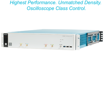
6 Series Low Profile Digitizer
LPD64 Datasheet
More Information
- 6 Series Low Profile Digitizer
- Product Support
- Explore more Software models
Read Online:
Performance in numbers
Input channels
- 4 SMA inputs
- Each SMA input supports Analog, Spectral (using DDC), or both simultaneously
Performance for every channel
- Sample Rate: 25 GS/s
- Bandwidth: DC to 8 GHz (optional)
- Vertical Resolution: 12-bit ADC
- Real-Time 2 GHz DDC (optional)
- Record Length: 125 Mpts (std), 250 Mpts, 500 Mpts or 1 Gpts (optional)
- Lowest-in-class Noise
- Highest-in-class ENOB
- Best-in-class channel-to-channel isolation
Real-Time Digital Down Converter (DDC)
- Patented individual time domain and frequency domain controls
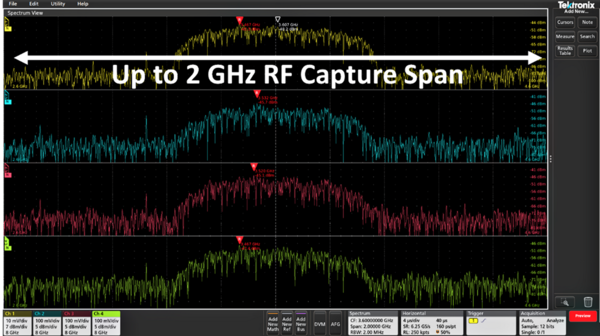
- Up to 2 GHz capture bandwidth (optional)
- IQ data transfers to PC for analysis (optional)
- Frequency vs time, Phase vs time and Magnitude vs time plotting (optional)
- RF vs Time Triggering (optional)
Superior low noise, vertical resolution and accuracy
- Low input noise enabled by new TEK061 front-end ASICs
- Noise at 1 mV/div: 54.8 uV @ 1 GHz
- Input Range: 10 mV to 10 V full scale
- DC Gain Accuracy: +/-1.0% at all gain settings >1 mV/div
- Effective Number of Bits (ENOB):
- 8.2 bits at 1 GHz
- 7.6 bits at 2.5 GHz
- 7.25 bits at 4 GHz
- 6.8 bits at 6 GHz
- 6.5 bits at 8 GHz
Remote communication and connectivity
- Ethernet 10/100/1000 port
- USB 3.0 device port (USBTMC) up to 800 Megabits/second
- LXI 1.5 Certified (VXI-11)
- Easy remote access with e*Scope; just enter the instrument IP address into a browser
- Award-winning user interface
- Connect a Mouse, Keyboard, Monitor or KVM switch
- Drivers: IVI-C, IVI-COM, LabVIEW, VOSS Scientific DAAAC
- Support for VISA, MATLAB, Python, C/C++/C#, Sockets
Measurement analysis
- 36 standard measurements
- Jitter Measurements (optional)
- User-Defined Filtering (optional)
- DDR Measurements (optional)
- Power Measurements (optional)
- Advanced Spectrum View (optional)
Operating systems
- Closed Embedded OS (standard)
- Microsoft Windows 10 (option 6-WINM2)
Security and declassification
- Password protect all user-accessible ports
- Settings to lock down the digitizer, prevents on-instrument user data storage
- Meets the needs for top secret and high security environments
Dimensions
- 2U (3.5 in./89 mm) tall & rack ready out of the box (standard configuration)
- 17 in. (432 mm) wide
- Fits into standard 24 - 32 in. (610 - 813 mm) racks
- Air flow is left to right for rack setup
With the lowest input noise and up to 8 GHz analog bandwidth, the 6 Series Low Profile Digitizer LPD64 provides the best signal fidelity for analyzing and debugging signals in a compact 2U rack space. With four SMA inputs each supporting Analog, Spectral (using DDC), or both simultaneously, lowest-in-class noise, and highest-in-class ENOB, the 6 Series Low Profile Digitizer LPD64 is ready for next generation test rack designs.
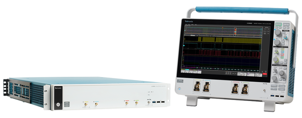
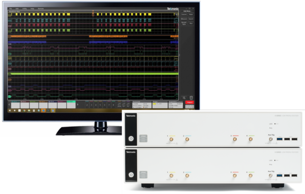
The 6 Series family
The 6 Series Low Profile Digitizer (LPD64) represents the highest performance digitizer on all channels in its class. This high-speed digitizer has the functionality of a digitizer and the power of an oscilloscope, sharing a similar hardware platform as the 6 Series MSO.
The transition from a 6 Series MSO benchtop oscilloscope to a Low Profile Digitizer has never been easier for R&D engineers needing to move their code, test work and platform performance into manufacturing and automation. Both products support the same user interface, remote capability, performance characteristics and programming back-end to make this transition as simple and easy as possible. No need to rewrite test routines and development test cycle code!
For more information on the capabilities of the benchtop 6 Series B MSO, including the award-winning user experience and the various analysis software options, please see the 6 Series B MSO datasheet at www.tek.com/6SeriesMSO.
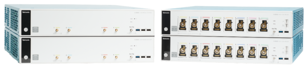
The Low Profile family
The 6 Series Low Profile Digitizer expands the performance of the 5 Series MSO Low Profile by adding twice the number of Tektronix TEK049 ASICS in the same 2U footprint. Now with 25 GS/s and up to 8 GHz on all channels. Low Profile users now have the choice of extreme high channel count or extreme performance in the same rack form factor.
For more information on the capabilities of the 5 Series MSO Low Profile (8 channels, 1 GHz), please see the datasheet at https://www.tek.com/MSO58LP/
| Quick Comparison | 6 Series Low Profile Digitizer | 5 Series MSO Low Profile Digitizer |
|---|---|---|
| Sample Rate | 25 GS/s | 6.25 GS/s |
| Analog Bandwidth | Up to 8 GHz | up to 1 GHz |
| RF (DDC) Span Bandwidth | 2 GHz | 500 MHz |
| ENOB @ 1 GHz | 8.2 bits | 7.6 bits |
| LXI compliance version | 1.5 | - |
| Rack Dimensions | 2U | 2U |
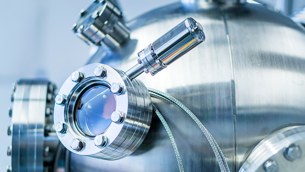
Machine diagnostics for physics
Physics is constantly leading the world to exciting new scientific discoveries in both matter and energy. These experiments require digitizers and oscilloscopes with improvements in precision, accuracy, performance and density when monitoring target test points. The 6 Series Low Profile Digitizer meets these requirements by bringing an industry leading performance, small form factor, Tektronix's class of reliability, easy remote accessibility, and award-winning user interface.
Common physics fields
- High Energy (Particle) Physics
- Nuclear Physics
- Atomic, Molecular and Optical Physics
- Condensed Matter
Research fields requiring single shot events or fast repetitive monitoring in their research labs; experiments like Photo Doppler Velocimetry (PDV), VISAR, gas guns, spectroscopy, accelerators and more. Many of these are diagnosing experiments and validating doppler shifts, phase alignments, beat frequencies, beam steering alignment or amplitudes. Doing this with reliable, high performance equipment is key for long term success.
Performance on every channel
Tired of turning on multiple digitizer channels and wondering what the sample rate, record length or bandwidth settings are? The 6 Series Low Profile Digitizer has industry leading performance on EVERY channel, always. No compromises!
Key performance features:
- 25 GS/s on ALL channels
- DC to 8 GHz on ALL channels
- Up to 1 Billion samples on ALL channels
- Up to 2 GHz RF DDC capture bandwidth on ALL channels
- 12-bit analog-to-digital converters
- Best-in-class low noise
- Best-in-class Effective Number Of Bits
- Best-in-class channel isolation (crosstalk)
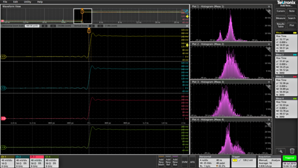
Spectrum View
It is often easier to debug an issue by viewing one or more signals in the frequency domain. Oscilloscopes and digitizers have included math-based FFTs for decades in an attempt to address this need. However, FFTs are notoriously difficult to use as they are driven by the same acquisition system that's delivering the analog time-domain view. When you optimize acquisition settings for the analog view, your frequency-domain view isn't what you want. When you get the frequency-domain view you want, your analog view is not what you want. With math-based FFTs, it is virtually impossible to get optimized views in both domains.
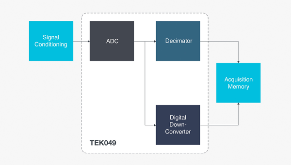
Spectrum View changes all of this. Tektronix' patented technology provides both a decimator for the time-domain and a digital down-converter for the frequency-domain behind each input. The two different acquisition paths let you simultaneously observe both time- and frequency-domain views of the input signal with independent acquisition settings for each domain. Other manufacturers offer various 'spectral analysis' packages that claim ease-of-use, but they all exhibit the limitations described above. Only Spectrum View provides both exceptional ease-of-use and the ability to achieve optimal views in both domains simultaneously.
Waveform and IQ data can easily be transferred from the 6 Series Low Profile to a PC using a variety of programming commands and API interfaces that come standard on all Tektronix 5 Series & 6 Series products.
Behind the performance
The Tektronix-designed TEK049 ASIC contains 12-bit analog-to-digital converters (ADCs) that provide 16 times more resolution than traditional 8-bit ADCs. The TEK049 is paired with the new Tektronix TEK061 front-end amplifier with industry leading low noise that enables the best signal fidelity possible to capture small signals with high resolution.
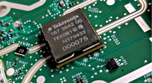
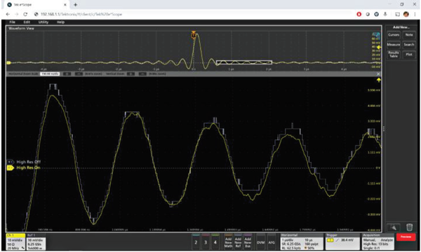
A key attribute to being able to view fine signal details on small, high-speed signals is noise. The higher a measurement systems' intrinsic noise, the less actual signal detail will be visible. This becomes more critical on a digitizer when the vertical settings are set to high sensitivity (like ≤ 10 mV/div) to view small signals that are prevalent in high-speed bus topologies. The 6 Series Low Profile has a new front-end ASIC, the TEK061, that enables breakthrough noise performance at the highest sensitivity settings.
In addition, a new High Res mode applies a hardware-based unique Finite Impulse Response (FIR) filter based on the selected sample rate. The FIR filter maintains the maximum bandwidth possible for that sample rate while preventing aliasing and removing noise from the digitizer amplifiers and ADC above the usable bandwidth for the selected sample rate. High Res mode always provides at least 12 bits of vertical resolution and extends all the way to 16 bits of vertical resolution at ≤ 625 MS/s sample rates and 200 MHz of bandwidth.
Building a next-generation test rack
Looking for a modern way to refresh your test rack, view, download or analyze your data? Looking to replace obsolete hardware without rewriting your code?
We understand that test rack designs take time and include numerous tradeoffs. Tektronix has heard your voice loud and clear and is blazing a new path to provide a richer set of tools to enable flexible ways to access data and replace obsolete hardware. If that means you’re automating a test rack with LabVIEW, Python or another interface, we have an expanding number of drivers and numerous support resources available.
Maybe you require an easy way to view waveforms on a remote computer. Not a problem, Tektronix has a software team designing new ways to control the instrument from a browser (E*Scope), store your data in the cloud (TekCloud), or stream data to our PC (TekScope). Providing modern age tools at your fingertips.
Lastly, users familiar with keyboards, mice, monitors, and KVM switches can continue to operate as they always have!

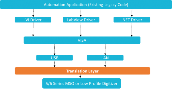
Upgrade Automated Test Equipment (ATE) systems quickly and smoothly
Was your automation code written in the 1970s, 1980s, or 1990s?
Anyone working closely with automated test systems knows that moving to a new model or platform can be painful. Modifying an existing codebase for a new product can be prohibitively expensive and complicated. Now there's a solution.
All 5 and 6 Series Low Profile instruments include a Programmatic Interface (PI) Translator. When enabled, the PI Translator acts as an intermediate layer between your test application and the digitizer. The PI translator recognizes a subset of legacy commands from the popular DPO/MSO5000B, DPO7000C, and DPO70000C oscilloscope platforms and translates them on the fly into supported commands. The interface is designed to be human-readable and easily extensible, which means that you can customize its behavior to minimize the amount of effort required when transitioning from obsolete instruments to the newest Tektronix platform.
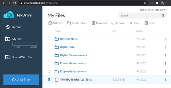
Access data in all the new ways you can dream about
Using TekDrive, you can upload, store, organize, search, download, and share any file type from any connected device. TekDrive is natively integrated into the 6 Series Low Profile instrument for seamless sharing and recalling of files - no USB stick is required. Analyze and explore standard files like .wfm, .isf, .tss, and .csv, directly in a browser with smooth interactive waveform viewers. TekDrive is purpose-built for integration, automation, and security. http://www.tekcloud.com/tekdrive

Get the analysis capability of an award-winning oscilloscope on your PC. Analyze waveforms anywhere, anytime. The basic license lets you view and analyze waveforms, perform many types of measurements and decode the most common serial buses - all while remotely accessing your oscilloscope. Advanced license options add capabilities such as multi-scope analysis, more serial bus decoding options, jitter analysis and power measurements. TekScope Multi-Scope enables you to connect and download data from up to 4 instruments (16-32 max channels) for easy viewing and cross-instrument analysis.
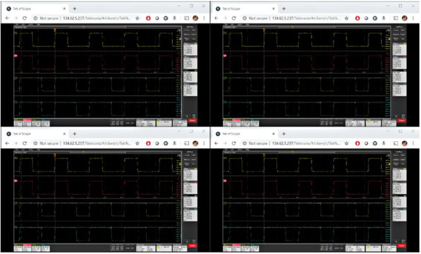
E*Scope is an easy method of viewing and controlling a 6 Series Low Profile instrument over a network connection in the same way that you do in-person with a monitor or keyboard. Simply type the instrument’s IP address into a browser to display the LXI landing page, then select the Instrument Control to access E*Scope. There are no drivers needed. It's all self-contained within the browser and you can control the instrument. It’s fast, responsive, and perfect for controlling or visualizing single or multiple instrument situations.
Synchronizing
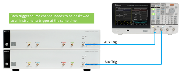
When synchronizing multiple instruments its important to have the smallest amount of skew between instrument channels to allow for data timing accuracy. Generally speaking this can be broken down into two types of skew; the part that comes from uncertainty between the aux trigger to analog channel, and the part that comes from trigger jitter. By calibrating out the effects of channel delay to the aux input we can reduce the amount of timing inaccuracy between instrument channels to just the jitter. This process is called deskewing an instrument.
Deskewing can be done to a reference channel that is simultaneously feeding a trigger edge (preferably over 1 Vpp) into the Aux Trigger input of multiple instruments and to the reference channel. When everything is adjusted, instrument to instrument channels can be within a very tight tolerance of only a couple sample points and within our specification of 200 ps. Whether you have 16 channels or 200 channels, all the data can be easily synchronized and analyzed.
Enhanced security
The 6 Series Low Profile Digitizer provides you with the option to protect company data through the Security menu. This includes the option to restrict access to the instrument by password-protecting remote network access, I/O ports, and firmware updates to ensure the security of the data. By default, the oscilloscope disables remote access on initial use and gives you the option to enable remote access with or without a password.
To clear user data, run TekSecure from the menu. Sanitize the oscilloscope by removing the SSD from the bottom of the instrument. 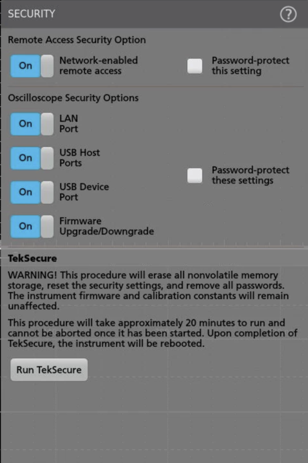
Arbitrary/Function Generator (AFG)
The instrument contains an optional integrated arbitrary/function generator, perfect for simulating sensor signals within a design or adding noise to signals to perform margin testing. The integrated function generator provides output of predefined waveforms up to MHz for sine, square, pulse, ramp/triangle, DC, noise, sin(x)/x (Sinc), Gaussian, Lorentz, exponential rise/fall, Haversine and cardiac. The AFG can load waveform records up to 128 k points in size from an internal file location or a USB mass storage device.
The AFG feature is compatible with Tektronix' ArbExpress PC-based waveform creation and editing software, making creation of complex waveforms fast and easy.
Digital Voltmeter (DVM) and Trigger Frequency Counter
The instrument contains an integrated 4-digit digital voltmeter (DVM) and 8-digit trigger frequency counter. Any of the analog inputs can be a source for the voltmeter, using the same probes that are already attached for general oscilloscope usage. The trigger frequency counter provides a very precise readout of the frequency of the trigger event on which you’re triggering.
Both the DVM and trigger frequency counter are available for free and are activated when you register your product.
User-defined filtering (optional)
In the broad sense, any system that processes a signal can be thought of as a filter. For example, an oscilloscope channel operates as a low pass filter where its 3 dB down point is referred to as its bandwidth. Given a waveform of any shape, a filter can be designed that can transform it into a defined shape within the context of some basic rules, assumptions, and limitations.
Digital filters have some significant advantages over analog filters. For example, the tolerance values of analog filter circuit components are high enough that high order filters are difficult or even impossible to implement. High order filters are easily implemented as digital filters. Digital filters can be implemented as Infinite Impulse Response (IIR) or Finite Impulse Response (FIR). The choice of IIR or FIR filters are based upon design requirements and application.
The 6 Series Low Profile has the ability to apply designated filters to math waveforms through a MATH arbitrary function. Option 6-UDFLT takes this functionality a level deeper, providing more than MATH arbitrary basic functions and adds flexibility to support standard filters and can be used for application centric filter designs.
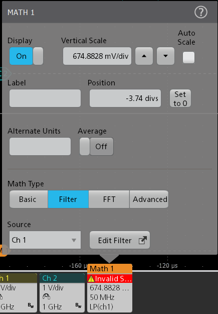
Filter types supported on the 6 Series Low Profile include:
- Low pass
- High pass
- Band pass
- Band stop
- All pass
- Hilbert
- Differentiator
- Custom
Filter response types supported on the 6 Series Low Profile include:
- Butterworth
- Chebyshev I
- Chebyshev II
- Elliptical
- Gaussian
- Bessel-Thomson
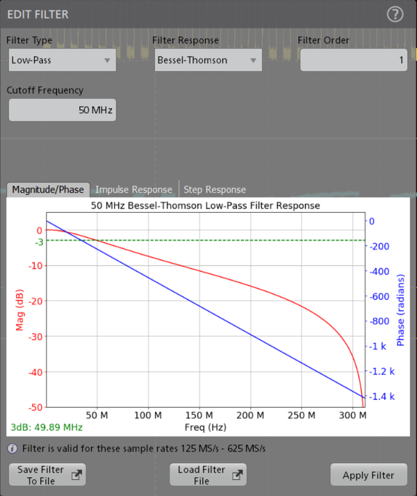
Filter designs can be saved, recalled, and applied once any editing has been completed.
Specifications
All specifications are guaranteed and apply to all models unless noted otherwise.
Model overview
| Characteristic | LPD64 |
|---|---|
| Analog inputs | 4 |
| Bandwidth (calculated rise time) | 1 GHz (400 ps), 2.5 GHz (160 ps), 4 GHz (100 ps), 6 GHz (66.67 ps), 8 GHz (50 ps) |
| DC Gain Accuracy | 50 Ω: ±2.0% 1, (±2.0% at 2 mV/div, ±4.0% at 1 mV/div, typical) 50 Ω: ±1.0% 2 of full scale, (±1.0% of full scale at 2 mV/div, ±2.0% at 1 mV/div, typical) |
| ADC Resolution | 12 bits |
| Vertical Resolution (all channels) | 8 bits @ 25 GS/s; 8 GHz 12 bits @ 12.5 GS/s; 4 GHz 13 bits @ 6.25 GS/s (High Res); 2 GHz 14 bits @ 3.125 GS/s (High Res); 1 GHz 15 bits @ 1.25 GS/s (High Res); 500 MHz 16 bits @ ≤625 MS/s (High Res); 200 MHz |
| Sample Rate | 25 GS/s on all channels |
| Record Length | 125 Mpoints on all channels (standard) 250 Mpoints, 500 Mpoints or 1 Gpoints on all channels (optional) |
| Waveform Capture Rate | >500,000 wfms/s (Peak Detect, Envelope acquisition mode), >30,000 wfms/s (all other acquisition modes) |
| Arbitrary/Function Generator (option) | 13 predefined waveform types with up to 50 MHz output |
| DVM | 4-digit DVM (free with product registration) |
| Trigger Frequency Counter | 8-digit frequency counter (free with product registration) |
Vertical system
- Input coupling
- DC
- Input impedance 50 Ω, DC coupled
- 50 Ω ±3%
- Input sensitivity range
- 50 Ω
- 1 mV/div to 1 V/div in a 1-2-5 sequence
- Note: 1 mV/div is a 2X digital zoom of 2 mV/div.
- Maximum input voltage
- 2.3VRMS, at < 100 mV/div, with peaks ≤±20 V (Pulse Width ≤ 1 us).
- 5.5VRMS, at ≥ 100 mV/div, with peaks ≤±20 V (Pulse Width ≤ 200 us)
- Effective bits (ENOB), typical
- 2 mV/div, High Res mode, 50 Ω, 10 MHz input with 90% full screen
Bandwidth ENOB 4 GHz 5.9 3 GHz 6.1 2.5 GHz 6.2 2 GHz 6.35 1 GHz 6.8 500 MHz 7.2 350 MHz 7.4 250 MHz 7.5 200 MHz 7.75 20 MHz 8.8 - 50 mV/div, High Res mode, 50 Ω, 10 MHz input with 90% full screen
Bandwidth ENOB 4 GHz 7.25 3 GHz 7.5 2.5 GHz 7.6 2 GHz 7.8 1 GHz 8.2 500 MHz 8.5 350 MHz 8.8 250 MHz 8.9 200 MHz 9 20 MHz 9.8 - 2 mV/div, Sample mode, 50 Ω, 10 MHz input with 90% full screen
Bandwidth ENOB 8 GHz 5.1 7 GHz 5.3 6 GHz 5.5 5 GHz 5.65 4 GHz 5.9 3 GHz 6.05 2.5 GHz 6.2 2 GHz 6.35 1 GHz 6.8 500 MHz 7.2 350 MHz 7.3 250 MHz 7.5 200 MHz 7.3 20 MHz 7.6 - 50 mV/div, Sample mode, 50 Ω, 10 MHz input with 90% full screen
Bandwidth ENOB 8 GHz 6.5 7 GHz 6.6 6 GHz 6.8 5 GHz 7 4 GHz 7.2 3 GHz 7.4 2.5 GHz 7.6 2 GHz 7.7 1 GHz 8.2 500 MHz 8.4 350 MHz 8.7 250 MHz 8.8 200 MHz 7.8 20 MHz 7.9
- DC balance
0.1 div with DC-50 Ω digitizer input impedance (50 Ω terminated)
0.2 div at 1 mV/div with DC-50 Ω digitizer input impedance (50 Ω terminated)
- Position range
- ±5 divisions
- Offset ranges, maximum
Input signal cannot exceed maximum input voltage for the 50 Ω input path.
Volts/div Setting Maximum offset range, 50 Ω Input 1 mV/div - 99 mV/div ±1 V 100 mV/div - 1 V/div ±10 V
- Offset accuracy
±(0.005 X | offset - position | + DC balance); Offset, position, and DC Balance in units of Volts
- Bandwidth selections
- 8 GHz model, 50 Ohm
- 20 MHz, 200 MHz, 250 MHz, 350 MHz, 500 MHz, 1 GHz, 2 GHz, 2.5 GHz, 3 GHz, 4 GHz, 5 GHz, 6 GHz, 7 GHz, and 8 GHz
- 6 GHz model, 50 Ohm
- 20 MHz, 200 MHz, 250 MHz, 350 MHz, 500 MHz, 1 GHz, 2 GHz, 2.5 GHz, 3 GHz, 4 GHz, 5 GHz, and 6 GHz
- 4 GHz model, 50 Ohm
- 20 MHz, 200 MHz, 250 MHz, 350 MHz, 500 MHz, 1 GHz, 2 GHz, 2.5 GHz, 3 GHz, and 4 GHz
- 2.5 GHz model, 50 Ohm
- 20 MHz, 200 MHz, 250 MHz, 350 MHz, 500 MHz, 1 GHz, 2 GHz, and 2.5 GHz
- 1 GHz model, 50 Ohm
- 20 MHz, 200 MHz, 250 MHz, 350 MHz, 500 MHz, and 1 GHz
- Bandwidth filtering optimized for
- Flatness or Step response
- Random noise, RMS, typical
- 50 Ω, typical
25 GS/s, Sample Mode, RMS V/div 1 mV/div 2 mV/div 5 mV/div 10 mV/div 20 mV/div 50 mV/div 100 mV/div 1 V/div 8 GHz 158 μV 158 μV 208 μV 342 μV 630 μV 1.49 mV 3.46 mV 29.7 mV 7 GHz 141 μV 143 μV 192 μV 311 μV 562 μV 1.31 mV 3.11 mV 26.2 mV 6 GHz 127 μV 127 μV 165 μV 274 μV 489 μV 1.18 mV 2.71 mV 23.6 mV 5 GHz 112 μV 113 μV 149 μV 239 μV 446 μV 1.05 mV 2.42 mV 21.1 mV 12.5 GS/s, HiRes Mode, RMS V/div 1 mV/div 2 mV/div 5 mV/div 10 mV/div 20 mV/div 50 mV/div 100 mV/div 1 V/div 4 GHz 97.4 μV 98.7 μV 124 μV 192 μV 344 μV 817 μV 1.92 mV 16.3 mV 3 GHz 82.9 μV 84 μV 105 μV 160 μV 282 μV 680 μV 1.62 mV 13.6 mV 2.5 GHz 76.5 μV 77.5 μV 93.8 μV 144 μV 257 μV 606 μV 1.44 mV 12.1 mV 2 GHz 68.1 μV 69.1 μV 83.6 μV 131 μV 226 μV 528 μV 1.28 mV 10.6 mV 1 GHz 54.8 μV 51.2 μV 63.4 μV 90.9 μV 160 μV 378 μV 941 μV 7.65 mV 500 MHz 39.7 μV 39.8 μV 48.1 μV 65.1 μV 115 μV 280 μV 666 μV 5.6 mV 350 MHz 33.8 μV 33.5 μV 40 μV 54.8 μV 94.3 μV 217 μV 560 μV 4.35 mV 250 MHz 30.8 μV 31.2 μV 36.1 μV 49.9 μV 80.3 μV 187 μV 482 μV 3.75 mV 200 MHz 25.3 μV 25.4 μV 29.7 μV 44 μV 70.7 μV 165 μV 445 μV 3.3 mV 20 MHz 8.68 μV 8.9 μV 10.4 μV 15.1 μV 27.5 μV 70.4 μV 158 μV 1.41 mV
- Crosstalk (channel isolation), typical
≥ -80 dB up to 2 GHz
≥ -65 dB up to 4 GHz
≥ -55 dB up to 8 GHz
for any two channels set to 200 mV/div.
Horizontal system
- Time base range
- 40 ps/div to 1,000 s/div
- Sample rate range
6.25 S/s to 25 GS/s (real time)
50 GS/s to 2.5 TS/s (interpolated)
- Record length range
All acquisition modes are 250 M maximum record length, down to 1 k minimum record length, adjustable in 1 sample increments.
Standard: 125 Mpoints
Option 6-RL-2: 250 Mpoints
- Seconds/Division range
Record length 1 K 10 K 100 K 1 M 10 M 62.5 M 125 M 250 M 500M 1 G Standard: 125 M 40 ps - 16 s 400 ps - 160 s 4 ns - 1000 s 2.5 μs - 1000 s 5 μs - 1000 s N/A N/A N/A Option 6-RL-2: 250 M 40 ps - 16 s 400 ps - 160 s 4 ps - 1000 s 2.5 μs - 1000 s 5 μs - 1000 s 10 μs - 1000 s N/A N/A Option 6-RL-3: 500 Mpts 40 ps - 16 s 400 ps - 160 s 4 ps - 1000 s 2.5 μs - 1000 s 5 μs - 1000 s 10 μs - 1000 s 20 us - 1000 s N/A Option 6-RL-4: 1 Gpts 40 ps - 16 s 400 ps - 160 s 4 ps - 1000 s 2.5 μs - 1000 s 5 μs - 1000 s 10 μs - 1000 s 20 us - 1000 s 40 us - 1000 s
- Aperture uncertainty (sample jitter)
Time duration Typical jitter <1 μs 80 fs <1 ms 130 fs
- Timebase accuracy
- ±1.0 x10⁻⁷ over any ≥1 ms time interval
Description Specification Factory Tolerance ±12 ppb; at calibration, 25 °C ambient, over any ≥1 ms interval Temperature stability ±20 ppb across the full operating range of 0 °C to 50 °C, after a sufficient soak time at the temperature; tested at operating temperatures Crystal aging ±300 ppb; frequency tolerance change at 25 °C over a period of 1 year
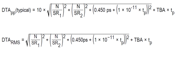
- Delta-time measurement accuracy, nominal

(assume edge shape that results from Gaussian filter response)
The formula to calculate delta-time measurement accuracy (DTA) for a given instrument setting and input signal assumes insignificant signal content above Nyquist frequency, where:
SR 1 = Slew Rate (1st Edge) around 1st point in measurement
SR 2 = Slew Rate (2nd Edge) around 2nd point in measurement
N = input-referred guaranteed noise limit (VRMS)
TBA = time base accuracy or reference frequency error
t p = delta-time measurement duration (sec)
- Maximum duration at highest sample rate
- 5 ms (standard) or 10 ms (option 6-RL-2, 250 Mpoints)
- Time base delay time range
- -10 divisions to 5,000 s
- Deskew range
- -125 ns to +125 ns with a resolution of 40 ps (for Peak Detect and Envelope acquisition modes).
- -125 ns to +125 ns with a resolution of 1 ps (for all other acquisition modes).
- Delay between analog channels, full bandwidth, typical
≤ 10 ps for any two channels with input impedance set to 50 Ω, DC coupling with equal Volts/div or above 10 mV/div
Trigger system
- Trigger modes
- Auto, Normal, and Single
- Trigger coupling
DC, HF Reject (attenuates > 50 kHz), LF Reject (attenuates < 50 kHz), noise reject (reduces sensitivity)
- Trigger holdoff range
- 0 ns to 10 seconds
- Trigger bandwidth (edge, pulse and logic), typical
Model Trigger type Trigger bandwidth 8 GHz Edge 8 GHz 8 GHz Pulse, Logic 4 GHz 6 GHz Edge 6 GHz 6 GHz Pulse, Logic 4 GHz 4 GHz, 2.5 GHz, 1 GHz: Edge, Pulse, Logic Product Bandwidth
- Edge-type trigger sensitivity, DC coupled, typical
Path Range Specification 50 Ω path 1 mV/div to 9.98 mV/div 3.0 div from DC to instrument bandwidth ≥ 10 mV/div < 1.0 division from DC to instrument bandwidth Line 90 V to 264 V line voltage at 50 - 60 Hz line frequency 103.5 V to 126.5 V
AUX Trigger in 250 mVPP, DC to 400 MHz
- Edge-type trigger sensitivity, not DC coupled, typical
Trigger Coupling Typical Sensitivity NOISE REJ 2.5 times the DC Coupled limits HF REJ 1.0 times the DC Coupled limits from DC to 50 kHz. Attenuates signals above 50 kHz. LF REJ 1.5 times the DC Coupled limits for frequencies above 50 kHz. Attenuates signals below 50 kHz.
- Trigger jitter, analog channels, typical
≤ 1.5 psRMS for sample mode and edge-type trigger
≤ 2 psRMS for edge-type trigger and FastAcq mode
≤ 40 psRMS for non edge-type trigger modes
- Trigger jitter, AUX input, typical
≤ 40 psRMS for sample mode and edge-type trigger
- AUX In trigger skew between instruments, typical
±100 ps jitter on each instrument with <450 ps skew; <550 ps total between instruments. Can be manually deskewed so channel-to-channel total skew is <200ps between instruments using AUX In.
Skew improves for pulse input voltages ≥1 Vpp
- Trigger level ranges
- This specification applies to logic and pulse thresholds.
Source Range Any Channel ±5 divs from center of screen Aux In Trigger ±5 V Line Fixed at about 50% of line voltage
- Trigger types
- Edge:
- Positive, negative, or either slope on any channel. Coupling includes DC, AC, noise reject, HF reject, and LF reject
- Pulse Width:
Trigger on width of positive or negative pulses. Event can be time- or logic-qualified
- Timeout:
- Trigger on an event which remains high, low, or either, for a specified time period. Event can be logic-qualified
- Runt:
- Trigger on a pulse that crosses one threshold but fails to cross a second threshold before crossing the first again. Event can be time- or logic-qualified
- Window:
- Trigger on an event that enters, exits, stays inside or stays outside of a window defined by two user-adjustable thresholds. Event can be time- or logic-qualified
- Logic:
- Trigger when logic pattern goes true, goes false, or occurs coincident with a clock edge. Pattern (AND, OR, NAND, NOR) specified for all input channels defined as high, low, or don't care. Logic pattern going true can be time-qualified
- Setup & Hold:
- Trigger on violations of both setup time and hold time between clock and data present on any input channels
- Rise / Fall Time:
- Trigger on pulse edge rates that are faster or slower than specified. Slope may be positive, negative, or either. Event can be logic-qualified
- Video:
- Trigger on all lines, odd, even, or all fields of NTSC, PAL, and SECAM video signals
- Sequence:
- Trigger on B event X time or N events after A trigger with a reset on C event. In general, A and B trigger events can be set to any trigger type with a few exceptions: logic qualification is not supported, if A event or B event is set to Setup & Hold, then the other must be set to Edge, and Ethernet and High Speed USB (480 Mbps) are not supported
- Visual trigger
- Qualifies standard triggers by scanning all waveform acquisitions and comparing them to on-screen areas (geometric shapes). An unlimited number of areas can be defined with In, Out, or Don't Care as the qualifier for each area. A boolean expression can be defined using any combination of visual trigger areas to further qualify the events that get stored into acquisition memory. Shapes include rectangle, triangle, trapezoid, hexagon and user-defined.
- Parallel Bus:
- Trigger on a parallel bus data value. Parallel bus can be from 1 to 4 bits (from the analog channels) in size. Supports Binary and Hex radices
- I2C Bus (option 6-SREMBD):
- Trigger on Start, Repeated Start, Stop, Address (7 or 10 bit), Data, or Address and Data on I2C buses up to 10 Mb/s
- I3C Bus (option 6-SRI3C)
- Trigger on Start, Repeated Start, Stop, Address, Data, I3C SDR Direct, I3C SDR Broadcast, Missing ACK, T-Bit Error, Broadcast Address Error, Hot-Join, HDR Restart, HDR Exit on I3C buses up to 10 Mb/s
- SPI Bus (option 6-SREMBD):
- Trigger on Slave Select, Idle Time, or Data (1-16 words) on SPI buses up to 20 Mb/s
- RS-232/422/485/UART Bus (option 6-SRCOMP):
- Trigger on Start Bit, End of Packet, Data, and Parity Error up to 15 Mb/s
- CAN Bus (option 6-SRAUTO):
- Trigger on Start of Frame, Type of Frame (Data, Remote, Error, or Overload), Identifier, Data, Identifier and Data, End Of Frame, Missing Ack, and Bit Stuff Error on CAN buses up to 1 Mb/s
- CAN FD Bus (option 6-SRAUTO):
- Trigger on Start of Frame, Type of Frame (Data, Remote, Error, or Overload), Identifier (Standard or Extended), Data (1-8 bytes), Identifier and Data, End Of Frame, Error (Missing Ack, Bit Stuffing Error, FD Form Error, Any Error) on CAN FD buses up to 16 Mb/s
- LIN Bus (option 6-SRAUTO):
- Trigger on Sync, Identifier, Data, Identifier and Data, Wakeup Frame, Sleep Frame, and Error on LIN buses up to 1 Mb/s
- FlexRay Bus (option 6-SRAUTO):
- Trigger on Start of Frame, Indicator Bits (Normal, Payload, Null, Sync, Startup), Frame ID, Cycle Count, Header Fields (Indicator Bits, Identifier, Payload Length, Header CRC, and Cycle Count), Identifier, Data, Identifier and Data, End Of Frame, and Errors on FlexRay buses up to 10 Mb/s
- SENT Bus (option 6-SRAUTOSEN)
- Trigger on Start of Packet, Fast Channel Status and Data, Slow Channel Message ID and Data, and CRC Errors
- SPMI Bus (option 6-SRPM):
- Trigger on Sequence Start Condition, Reset, Sleep, Shutdown, Wakeup, Authenticate, Master Read, Master Write, Register Read, Register Write, Extended Register Read, Extended Register Write, Extended Register Read Long, Extended Register Write Long, Device Descriptor Block Master Read, Device Descriptor Block Slave Read, Register 0 Write, Transfer Bus Ownership, and Parity Error
- USB 2.0 LS/FS/HS Bus (option 6-SRUSB2):
- Trigger on Sync, Reset, Suspend, Resume, End of Packet, Token (Address) Packet, Data Packet, Handshake Packet, Special Packet, Error on USB buses up to 480 Mb/s
- Ethernet Bus (option 6-SRENET):
- Trigger on Start of Frame, MAC Addresses, MAC Q-tag, MAC Length/Type, MAC Data, IP Header, TCP Header, TCP/IPV4 Data, End of Packet, and FCS (CRC) Error on 10BASE-T and 100BASE-TX buses
- Audio (I2S, LJ, RJ, TDM) Bus (option 6-SRAUDIO):
- Trigger on Word Select, Frame Sync, or Data. Maximum data rate for I2S/LJ/RJ is 12.5 Mb/s. Maximum data rate for TDM is 25 Mb/s
- MIL-STD-1553 Bus (option 6-SRAERO):
- Trigger on Sync, Command (Transmit/Receive Bit, Parity, Subaddress / Mode, Word Count / Mode Count, RT Address), Status (Parity, Message Error, Instrumentation, Service Request, Broadcast Command Received, Busy, Subsystem Flag, Dynamic Bus Control Acceptance, Terminal Flag), Data, Time (RT/IMG), and Error (Parity Error, Sync Error, Manchester Error, Non-contiguous Data) on MIL-STD-1553 buses
- ARINC 429 Bus (option 6-SRAERO):
- Trigger on Word Start, Label, Data, Label and Data, Word End, and Error (Any Error, Parity Error, Word Error, Gap Error) on ARINC 429 buses up to 1 Mb/s
- RF Magnitude vs. Time and RF Frequency vs. Time (option 6-SV-RFVT):
- Trigger on edge, pulse width and timeout events
Acquisition system
- Sample
- Acquires sampled values
- Peak Detect
- Captures glitches as narrow as 160 ps at all sweep speeds
- Averaging
- From 2 to 10,240 waveforms
- Maximum averaging speed = 180 waveforms/s
- Fast Hardware Averaging
- An acquisition mode for acquiring a large number of averages in a short amount of time. Fast hardware averaging optimizes the acquisition path, reducing storage truncation error and smoothing out fine scale non-linearity imperfections via an optional offset dithering technique. This feature is available through programmatic interface commands.
- From 2 to 1,000,000 waveforms
- Maximum averaging speed = 32,000 waveforms/s
- Envelope
- Min-max envelope reflecting Peak Detect data over multiple acquisitions
- High Res
Applies a unique Finite Impulse Response (FIR) filter for each sample rate that maintains the maximum bandwidth possible for that sample rate while preventing aliasing and removing noise from the oscilloscope amplifiers and ADC above the usable bandwidth for the selected sample rate.
High Res mode always provides at least 12 bits of vertical resolution and extends all the way to 16 bits of vertical resolution at ≤ 625 MS/s sample rates.
- FastAcq®
FastAcq optimizes the instrument for analysis of dynamic signals and capture of infrequent events.
Maximum waveform capture rate:
- >500,000 wfms/s (Peak Detect or Envelope Acquisition mode)
- >30,000 wfms/s (All other acquisition modes)
- Roll mode
- Scrolls sequential waveform points across the display in a right-to-left rolling motion, at timebase speeds of 40 ms/div and slower, when in Auto trigger mode.
- History mode
- Makes use of the maximum record length, allowing you to capture many triggered acquisitions, stop when you see something of interest, and quickly review all stored triggered acquisitions.
The number of available acquisitions stored in history is (Maximum record length) / (Current record length setting).
- FastFrame™
Acquisition memory divided into segments.
Maximum trigger rate >5,000,000 waveforms per second
Minimum frame size = 50 points
Maximum Number of Frames: For frame size ≥ 1,000 points, maximum number of frames = record length / frame size.
For 50 point frames, maximum number of frames = 1,000,000
Waveform measurements
- Cursor types
- Waveform, V Bars, H Bars, V&H Bars, and Polar (XY/XYZ plots only)
- DC voltage measurement accuracy, Average acquisition mode
Measurement Type DC Accuracy (In Volts) Average of ≥ 16 waveforms ±((DC Gain Accuracy) * |reading - (offset - position)| + Offset Accuracy + 0.05 * V/div setting) Delta volts between any two averages of ≥ 16 waveforms acquired with the same oscilloscope setup and ambient conditions ±(DC Gain Accuracy * |reading| + 0.1 div)
- Automatic measurements
- 36, of which an unlimited number can be displayed as either individual measurement badges or collectively in a measurement results table
- Amplitude measurements
- Amplitude, Maximum, Minimum, Peak-to-Peak, Positive Overshoot, Negative Overshoot, Mean, RMS, AC RMS, Top, Base, and Area
- Timing measurements
- Period, Frequency, Unit Interval, Data Rate, Positive Pulse Width, Negative Pulse Width, Skew, Delay, Rise Time, Fall Time, Phase, Rising Slew Rate, Falling Slew Rate, Burst Width, Positive Duty Cycle, Negative Duty Cycle, Time Outside Level, Setup Time, Hold Time, Duration N-Periods, High Time, Low Time, Time to Minimum, and Time to Maximum
- Jitter measurements (standard)
- TIE and Phase Noise
- Measurement statistics
- Mean, Standard Deviation, Maximum, Minimum, and Population. Statistics are available on both the current acquisition and all acquisitions
- Reference levels
- User-definable reference levels for automatic measurements can be specified in either percent or units. Reference levels can be set to global for all measurements, per source channel or signal, or unique for each measurement
- Gating
- Screen, Cursors, Logic, Search, or Time. Specifies the region of an acquisition in which to take measurements. Gating can be set to Global (affects all measurements set to Global) or Local (all measurements can have a unique Time gate setting; only one Local gate is available for Screen, Cursors, Logic, and Search actions).
- Measurement plots
- Histogram, Time Trend, Spectrum, Eye Diagram (TIE measurement only), Phase Noise (Phase Noise measurement only)
- Fast eye rendering: Shows the Unit Intervals (UIs) that define the boundaries of the eye along with a user specified number of surrounding UIs for added visual context
- Complete eye rendering: Shows all valid Unit Intervals (UIs)
- Measurement limits
- Pass/fail testing for user-definable limits on measurement values. Act on event for measurement value failures include Save Screen Capture, Save Waveform, System Request (SRQ), and Stop Acquisitions
- Jitter analysis (option 6-DJA) adds the following:
- Measurements
Jitter Summary, TJ@BER, RJ- δδ, DJ- δδ, PJ, RJ, DJ, DDJ, DCD, SRJ, J2, J9, NPJ, F/2, F/4, F/8, Eye Height, Eye Height@BER, Eye Width, Eye Width@BER, Eye High, Eye Low, Q-Factor, Bit High, Bit Low, Bit Amplitude, DC Common Mode, AC Common Mode (Pk-Pk), Differential Crossover, T/nT Ratio, SSC Freq Dev, SSC Modulation Rate
- Measurement plots
- Digital power management (option 6-DPM) adds the following:
- Eye Diagram and Jitter Bathtub
- Fast eye rendering: Shows the Unit Intervals (UIs) that define the boundaries of the eye along with a user specified number of surrounding UIs for added visual context
- Complete eye rendering: Shows all valid Unit Intervals (UIs)
- Measurement limits
Pass/fail testing for user-definable limits on measurement values. Act on event for measurement value failures include Save Screen Capture, Save Waveform, System Request (SRQ), and Stop Acquisitions
- Eye diagram mask testing
Automated mask pass/fail testing
- Power analysis (option 6-PWR) adds the following:
- Measurements
Input Analysis (Frequency, VRMS, IRMS, voltage and current Crest Factors, True Power, Apparent Power, Reactive Power, Power Factor, Phase Angle, Harmonics, Inrush Current, Input Capacitance )
Amplitude Analysis (Cycle Amplitude, Cycle Top, Cycle Base, Cycle Maximum, Cycle Minimum, Cycle Peak-to-Peak)
Timing Analysis (Period, Frequency, Negative Duty Cycle, Positive Duty Cycle, Negative Pulse Width, Positive Pulse Width)
Switching Analysis (Switching Loss, dv/dt, di/dt, Safe Operating Area, RDSon)
Magnetic Analysis (Inductance, I vs. Intg(V), Magnetic Loss, Magnetic Property)
Output Analysis (Line Ripple, Switching Ripple, Efficiency, Turn-on Time, Turn-off Time)
Frequency Response Analysis (Control Loop Response Bode Plot, Power Supply Rejection Ratio, Impedance)
- Measurement Plots
- Harmonics Bar Graph, Switching Loss Trajectory Plot, and Safe Operating Area
- Digital Power Management (option 6-DPM) adds the following:
- Measurements
Ripple Analysis (Ripple)
Transient Analysis (Overshoot, Undershoot, Turn On Overshoot, DC Rail Voltage)
Power Sequence Analysis (Turn-on, Turn-off)
Jitter Analysis (TIE, PJ, RJ, DJ, Eye Height, Eye Width, Eye High, Eye Low)
Power Supply Induced Jitter (PSIJ)
- DDR3/LPDDR3 memory debug and analysis option (6-DBDDR3) adds the following:
- Measurements
Amplitude Measurements (AOS, AUS, Vix(ac), AOS Per tCK, AUS Per tCK, AOS Per UI, AUS Per UI)
Time Measurements (tRPRE, tWPRE, tPST, Hold Diff, Setup Diff, tCH(avg), tCK(avg), tCL(avg), tCH(abs), tCL(abs), tJIT(duty), tJIT(per), tJIT(cc), tERR(n), tERR(m-n), tDQSCK, tCMD-CMD, tCKSRE, tCKSRX)
- LVDS debug and analysis option (option 6-DBLVDS) adds the following:
- Data Lane Measurements
Generic Test (Unit Interval, Rise Time, Fall Time, Data Width, Data Intra Skew (PN), Data Inter Skew (Lane-to-Lane), Data Peak-to-Peak)
Jitter Test (AC Timing, Clock Data Setup Time, Clock Data Hold Time, Eye Diagram (TIE), TJ@BER, DJ Delta, RJ Delta, DDJ, De-Emphasis Level)
- Clock Lane Measurements
Generic Test (Frequency, Period, Duty Cycle, Rise Time, Fall Time, Clock Intra Skew (PN), Clock Peak-to-Peak)
Jitter Test (TIE, DJ, RJ)
SSC On (Mod Rate, Frequency Deviation Mean)
Waveform math
- Number of math waveforms
- Unlimited
- Arithmetic
- Add, subtract, multiply, and divide waveforms and scalars
- Algebraic expressions
- Define extensive algebraic expressions including waveforms, scalars, user-adjustable variables, and results of parametric measurements. Perform math on math using complex equations. For example (Integral (CH1 - Mean(CH1)) X 1.414 X VAR1)
- Math functions
- Invert, Integrate, Differentiate, Square Root, Exponential, Log 10, Log e, Abs, Ceiling, Floor, Min, Max, Degrees, Radians, Sin, Cos, Tan, ASin, ACos, and ATan
- Relational
- Boolean result of comparison >, <, ≥, ≤, =, and ≠
- Logic
- AND, OR, NAND, NOR, XOR, and EQV
- Filtering function (standard)
- Loading of user-definable filters. Users specify a file containing the coefficients of the filter.
- Filtering function (option 6-UDFLT)
- Filter types
- Low pass, High pass, Band pass, Band stop, All pass, Hilbert, Differentiator, and Custom
- Filter response types
- Butterworth, Chebyshev I, Chebyshev II, Elliptical, Gaussian, and Bessel-Thomson
- FFT functions
- Spectral Magnitude and Phase, and Real and Imaginary Spectra
- FFT vertical units
Magnitude: Linear and Log (dBm)
Phase: Degrees, Radians, and Group Delay
- FFT window functions
- Hanning, Rectangular, Hamming, Blackman-Harris, Flattop2, Gaussian, Kaiser-Bessel, and TekExp
Spectrum View
- Center Frequency
- Limited by instrument analog bandwidth
- Span
- 74.5 Hz – 1.25 GHz (Standard)
74.5 Hz – 2 GHz (option 6-SV-BW-1)
Coarse adjustment in a 1-2-5 sequence
- RF Measurements
- Channel Power (CHP), Adjacent Channel Power Ratio (ACPR), and Occupied Bandwidth (OBW) measurements on Spectrum View trace data and display
- RF vs. Time Traces
- Magnitude vs. time, Frequency vs. time, Phase vs. time (with option 6-SV-RFVT)
- RF vs. Time Trigger
- Edge, pulse width, and timeout trigger on RF Magnitude vs. Time and RF Frequency vs. Time (with option 6-SV-RFVT)
- Spectrograms
- RF Frequency vs. Time vs. Amplitude display with frequency on x-axis, time on y-axis, and power level indicated by variations in color (with option 6-SV-RFVT)
- Resolution Bandwidth (RBW)
93 μHz to 62.5 MHz
93 μHz to 100 MHz (with option 6-SV-BW-1)
- IQ capture
- The data is stored as in-phase and quadrature (I&Q) samples and precise synchronization is maintained between the time domain data and the I&Q data.
- When RF vs. Time traces are activated (with option 6-SV-RFVT), IQ data can be captured and exported to file for more analysis within 3rd party applications.
- The max acquisition time varies with span and sample rate. At 25 GS/s and 2 GHz span, the max acquisition time is 0.086 seconds. For 1 GHz span, the max acquisition time is 0.172 seconds. For 40 MHz span, the max acquisition time is 2.749 seconds. For 1 MHz span, the max acquisition time is 87.961 seconds.
- Window types and factors
Window type Factor Blackman-Harris 1.90 Flat-Top 2 3.77 Hamming 1.30 Hanning 1.44 Kaiser-Bessel 2.23 Rectangular 0.89
- Spectrum Time
- FFT Window Factor / RBW
- Reference level
- Reference level is automatically set by the analog channel Volts/div setting
- Setting range: -42 dBm to +44 dBm
- Vertical Position
- -100 divs to +100 divs
- Vertical units
- dBm, dBµW, dBmV, dBµV, dBmA, dBµA
- Horizontal scaling
- Linear, Log
- Multi-channel spectrum analysis
- Each FlexChannel input can be configured with Spectrum View, RF vs. Time traces (with option RFVT), and Spectrogram (with option RFVT).
- Multiple RF measurements can be performed simultaneously across channels.
- Spectrum Time and Center Frequency settings can be unlocked and moved independently from each other across channels. All Spectrum View channels must share the same Span, Resolution Bandwidth and Window Type.
Search
- Number of searches
- Unlimited
- Search types
- Search through long records to find all occurrences of user specified criteria including edges, pulse widths, timeouts, runt pulses, window violations, logic patterns, setup & hold violations, rise/fall times, and bus protocol events. Search results can be viewed in the Waveform View or in the Results table.
Save
- Waveform type
- Tektronix Waveform Data (.wfm), Comma Separated Values (.csv), MATLAB (.mat)
- Waveform gating
- Cursors, Screen, Resample (save every nth sample)
- Screen capture type
- Portable Network Graphic (*.png), 24-bit Bitmap (*.bmp), JPEG (*.jpg)
- Setup type
- Tektronix Setup (.set)
- Report type
- Adobe Portable Documents (.pdf), Single File web Pages (.mht)
- Session type
- Tektronix Session Setup (.tss)
Display (available only through the video out ports or e*Scope)
- Display type
- External monitor
- Display resolution
- 1,920 horizontal × 1,080 vertical pixels (High Definition)
- Display modes
Overlay: traditional oscilloscope display where traces overlay each other
Stacked: display mode where each waveform is placed in its own slice and can take advantage of the full ADC range while still being visually separated from other waveforms. Groups of channels can also be overlaid within a slice to simplify visual comparison of signals.
- Zoom
- Horizontal and vertical zooming is supported in all waveform and plot views.
- Interpolation
- Sin(x)/x and Linear
- Waveform styles
- Vectors, dots, variable persistence, and infinite persistence
- Graticules
- Movable and fixed graticules, selectable between Grid, Time, Full, and None
- Color palettes
Normal and inverted for screen captures
Individual waveform colors are user-selectable
- Format
- YT, XY, and XYZ
- Local Language User Interface
- English, Japanese, Simplified Chinese, Traditional Chinese, French, German, Italian, Spanish, Portuguese, Russian, Korean
- Local Language Help
- English, Japanese, Simplified Chinese
Arbitrary-Function Generator (optional)
- Function types
- Arbitrary, sine, square, pulse, ramp, triangle, DC level, Gaussian, Lorentz, exponential rise/fall, sin(x)/x, random noise, Haversine, Cardiac
- Amplitude range
- Values are peak-to-peak voltages
Waveform 50 Ω 1 MΩ Arbitrary 10 mV to 2.5 V 20 mV to 5 V Sine 10 mV to 2.5 V 20 mV to 5 V Square 10 mV to 2.5 V 20 mV to 5 V Pulse 10 mV to 2.5 V 20 mV to 5 V Ramp 10 mV to 2.5 V 20 mV to 5 V Triangle 10 mV to 2.5 V 20 mV to 5 V Gaussian 10 mV to 1.25 V 20 mV to 2.5 V Lorentz 10 mV to 1.2 V 20 mV to 2.4 V Exponential Rise 10 mV to 1.25 V 20 mV to 2.5 V Exponential Fall 10 mV to 1.25 V 20 mV to 2.5 V Sine(x)/x 10 mV to 1.5 V 20 mV to 3.0 V Random Noise 10 mV to 2.5 V 20 mV to 5 V Haversine 10 mV to 1.25 V 20 mV to 2.5 V Cardiac 10 mV to 2.5 V 20 mV to 5 V
- Sine waveform
- Frequency range
- 0.1 Hz to 50 MHz
- Frequency setting resolution
- 0.1 Hz
- Frequency accuracy
- 130 ppm (frequency ≤ 10 kHz), 50 ppm (frequency > 10 kHz)
This is for Sine, Ramp, Square and Pulse waveforms only.
- Amplitude range
- 20 mVpp to 5 Vpp into Hi-Z; 10 mVpp to 2.5 Vpp into 50 Ω
- Amplitude flatness, typical
±0.5 dB at 1 kHz
±1.5 dB at 1 kHz for < 20 mVpp amplitudes
- Total harmonic distortion, typical
1% for amplitude ≥ 200 mVpp into 50 Ω load
2.5% for amplitude > 50 mV AND < 200 mVpp into 50 Ω load
This is for Sine wave only.
- Spurious free dynamic range, typical
40 dB (Vpp ≥ 0.1 V); 30 dB (Vpp ≥ 0.02 V), 50 Ω load
- Square and pulse waveform
- Frequency range
- 0.1 Hz to MHz
- Frequency setting resolution
- 0.1 Hz
- Frequency accuracy
- 130 ppm (frequency ≤ 10 kHz), 50 ppm (frequency > 10 kHz)
- Amplitude range
- 20 mVpp to 5 Vpp into Hi-Z; 10 mVpp to 2.5 Vpp into 50 Ω
- Duty cycle range
- 10% - 90% or 10 ns minimum pulse, whichever is larger
- Minimum pulse time applies to both on and off time, so maximum duty cycle will reduce at higher frequencies to maintain 10 ns off time
- Duty cycle resolution
- 0.1%
- Minimum pulse width, typical
- 10 ns. This is the minimum time for either on or off duration.
- Rise/Fall time, typical
- 5 ns, 10% - 90%
- Pulse width resolution
- 100 ps
- Overshoot, typical
- < 6% for signal steps greater than 100 mVpp
- This applies to overshoot of the positive-going transition (+overshoot) and of the negative-going (-overshoot) transition
- Asymmetry, typical
- ±1% ±5 ns, at 50% duty cycle
- Jitter, typical
- < 60 ps TIERMS, ≥ 100 mVpp amplitude, 40%-60% duty cycle
- Ramp and triangle waveform
- Frequency range
- 0.1 Hz to
- Frequency setting resolution
- 0.1 Hz
- Frequency accuracy
- 130 ppm (frequency ≤ 10 kHz), 50 ppm (frequency > 10 kHz)
- Amplitude range
- 20 mVpp to 5 Vpp into Hi-Z; 10 mVpp to 2.5 Vpp into 50 Ω
- Variable symmetry
- 0% - 100%
- Symmetry resolution
- 0.1%
- DC level range
±2.5 V into Hi-Z
±1.25 V into 50 Ω
- Random noise amplitude range
20 mVpp to 5 Vpp into Hi-Z
10 mVpp to 2.5 Vpp into 50 Ω
- Sin(x)/x
- Maximum frequency
- MHz
- Gaussian pulse, Haversine, and Lorentz pulse
- Maximum frequency
- MHz
- Lorentz pulse
- Frequency range
- 0.1 Hz to MHz
- Amplitude range
- 20 mVpp to 2.4 Vpp into Hi-Z
10 mVpp to 1.2 Vpp into 50 Ω
- Cardiac
- Frequency range
- 0.1 Hz to
- Amplitude range
- 20 mVpp to 5 Vpp into Hi-Z
10 mVpp to 2.5 Vpp into 50 Ω
- Arbitrary
- Memory depth
- 1 to 128 k
- Amplitude range
- 20 mVpp to 5 Vpp into Hi-Z
10 mVpp to 2.5 Vpp into 50 Ω
- Repetition rate
- 0.1 Hz to MHz
- Sample rate
- 250 MS/s
- Signal amplitude accuracy
- ±[ (1.5% of peak-to-peak amplitude setting) + (1.5% of absolute DC offset setting) + 1 mV ] (frequency = 1 kHz)
- Signal amplitude resolution
1 mV (Hi-Z)
500 μV (50 Ω)
- Sine and ramp frequency accuracy
130 ppm (frequency ≤10 kHz)
50 ppm (frequency >10 kHz)
- DC offset range
±2.5 V into Hi-Z
±1.25 V into 50 Ω
- DC offset resolution
1 mV (Hi-Z)
500 μV (50 Ω)
- DC offset accuracy
±[ (1.5% of absolute offset voltage setting) + 1 mV ]
Add 3 mV of uncertainty per 10 °C change from 25 °C ambient
Digital volt meter (DVM)
- Measurement types
DC, ACRMS+DC, ACRMS, Trigger frequency count
- Voltage resolution
- 4 digits
- Voltage accuracy
- DC:
±((1.5% * |reading - offset - position|) + (0.5% * |(offset - position)|) + (0.1 * Volts/div))
De-rated at 0.100%/°C of |reading - offset - position| above 30 °C
Signal ± 5 divisions from screen center
- AC:
± 3% (40 Hz to 1 kHz) with no harmonic content outside 40 Hz to 1 kHz range
AC, typical: ± 2% (20 Hz to 10 kHz)
For AC measurements, the input channel vertical settings must allow the VPP input signal to cover between 4 and 10 divisions and must be fully visible on the screen
Trigger frequency counter
- Resolution
- 8-digits
- Accuracy
±(1 count + time base accuracy * input frequency)
The signal must be at least 8 mVpp or 2 div, whichever is greater.
- Maximum input frequency
- 10 Hz to maximum bandwidth of the analog channel
- The signal must be at least 8 mVpp or 2 div, whichever is greater.
Processor system
- Host processor
- Intel i5-4400E, 2.7 GHz, 64-bit, dual core processor, 8 GB system RAM
- Operating system
Closed Embedded OS (std configuration). No access to OS file system.
Instrument with option 6-WINM2 installed: Microsoft Windows 10
- Internal storage
- ≥ 80 GB. Form factor is an 80 mm m.2 card with a SATA-3 interface
512 GB m.2 drive with a SATA-3 interface (with option 6-WINM2)
Input-Output ports
- DisplayPort connector
- A 20-pin DisplayPort connector; connect to show the oscilloscope display on an external monitor or projector
- DVI connector
A 29-pin DVI-I connector; connect to show the oscilloscope display on an external monitor or projector
- VGA
DB-15 female connector; connect to show the oscilloscope display on an external monitor or projector
- Probe compensator signal, typical
- Connection:
- Connectors are located on the lower front right of the instrument
- Amplitude:
- 0 to 2.5 V
- Frequency:
- 1 kHz
- Source impedance:
- 1 kΩ
- External reference input
The time-base system can phase lock to an external 10 MHz reference signal .
There are two ranges for the reference clock.
The instrument can accept a high-accuracy reference clock of 10 MHz ±2 ppm or a lower-accuracy reference clock of 10 MHz ±1 kppm.
- USB interface (Host, Device ports)
- Front panel USB Host ports: Two USB 2.0 Hi-Speed ports, one USB 3.0 SuperSpeed port
- Rear panel USB Host ports: Two USB 2.0 Hi-Speed ports, two USB 3.0 SuperSpeed ports
- Rear panel USB Device port: One USB 3.0 SuperSpeed Device port providing USBTMC support
- Ethernet interface
- 10/100/1000 Mb/s
- Auxiliary output
Rear-panel BNC connector. Output can be configured to provide a positive or negative pulse out when the oscilloscope triggers, the internal oscilloscope reference clock out, or an AFG sync pulse
Characteristic Limits Vout (HI) ≥ 2.5 V open circuit; ≥ 1.0 V into a 50 Ω load to ground Vout (LO) ≤ 0.7 V into a load of ≤ 4 mA; ≤0.25 V into a 50 Ω load to ground
- Kensington-style lock
- Rear-panel security slot connects to standard Kensington-style lock
- LXI
Class: LXI Core 2016
Version: 1.5
Power source
- Power
- Power consumption
360 Watts maximum
- Source voltage
- 100 - 240 V ±10% at 50 Hz to 60 Hz
- 115 V ±10% at 400 Hz
Physical characteristics
- Dimensions
Height: 3.44 in (87.3 mm)
Width: 17.01 in (432 mm)
Depth: 23.85 in (605.7 mm)
Fits rack depths from 24 inches to 32 inches
- Weight
- 29.4 lbs (13.34 kg)
- Cooling
- The clearance requirement for adequate cooling is 2.0 in (50.8 mm) on the left and right sides of the instrument. Air flows from left to right through the instrument.
- Rackmount configuration
- 2U rack mount kit is included as standard configuration
Environmental specifications
- Temperature
- Operating
- +0 °C to +50 °C (32 °F to 122 °F)
- Non-operating
- -20 °C to +60 °C (-4 °F to 140 °F)
- Humidity
- Operating
- 5% to 90% relative humidity (% RH) at up to +40 °C
- 5% to 55% RH above +40 °C up to +50 °C, noncondensing
- Non-operating
- 5% to 90% relative humidity (% RH) at up to +60 °C, noncondensing
- Altitude
- Operating
- Up to 3,000 meters (9,843 feet)
- Non-operating
- Up to 12,000 meters (39,370 feet)
- Temperature
- Operating
- +0 °C to +50 °C (32 °F to 122 °F)
- Non-operating
- Humidity
- Operating
5% to 90% relative humidity (% RH) at up to +40 °C
5% to RH above +40 °C up to +50 °C, noncondensing
- Altitude
- Operating
- Up to 3,000 meters (9,843 feet)
- Non-operating
- Up to 12,000 meters (39,370 feet)
EMC, Environmental, and Safety
- Safety certification
- US NRTL Listed - UL61010-1 and UL61010-2-030
- Canadian Certification - CAN/CSA-C22.2 No. 61010.1 and CAN/CSA-C22.2 No 61010.2.030
- EU Compliance - Low Voltage Directive 2014-35-EU and EN61010-1.
- International Compliance - IEC 61010-1 and IEC61010-2-030
- Regulatory
CE marked for the European Union and CSA approved for the USA and Canada
RoHS compliant
Software
- IVI driver
Provides a standard instrument programming interface for common applications such as LabVIEW, LabWindows/CVI, Microsoft .NET, and MATLAB. Compatible with Python, C/C++/C# and many other languages through VISA.
- e*Scope®
Enables control of the oscilloscope over a network connection through a standard web browser. Simply enter the IP address or network name of the oscilloscope and a web page will be served to the browser. Transfer and save settings, waveforms, measurements, and screen images or make live control changes to settings on the oscilloscope directly from the web browser. Optionally configure e*Scope authentication to password protect access to control and view the oscilloscope.
- LXI Web interface
Connect to the oscilloscope through a standard Web browser by simply entering the oscilloscope's IP address or network name in the address bar of the browser. The Web interface enables viewing of instrument status and configuration, status and modification of network settings, and instrument control through the e*Scope web-based remote control.All web interaction conforms to LXI specification, version 1.5.
- Programming Examples
Programming with the 4/5/6 Series platforms has never been easier. With a programmers manual and a GitHub site you have many commands and examples to help you get started remotely automating your instrument. See https://github.com/tektronix/programmatic-control-examples.
Ordering Information
Use the following steps to select the appropriate instrument and options for your measurement needs.
Step 1
- Start by selecting the model.
Model Number of channels LPD64 4
- Each model includes
- Rackmount attachments installed
- Installation and safety manual
- Embedded Help
- Power cord
- Calibration certificate documenting traceability to National Metrology Institute(s) and ISO9001/ISO17025 quality system registration
- One-year warranty covering all parts and labor on the instrument.
Step 2
- Configure your Low Profile Digitizer by selecting the analog channel bandwidth you need
- Choose the bandwidth you need today by choosing one of these bandwidth options. You can upgrade it later by purchasing an upgrade option.
Bandwidth Option Bandwidth 6-BW-1000 1 GHz 6-BW-2500 2.5 GHz 6-BW-4000 4 GHz 6-BW-6000 6 GHz 6-BW-8000 8 GHz
Step 3
- Add instrument functionality
Instrument functionality can be ordered with the instrument or later as an upgrade kit.
Instrument option Built-in functionality 6-RL-2 Extend record length from 125 Mpts/channel to 250 Mpts/channel 6-RL-3 Extend record length from 125 Mpts/channel to 500 Mpts/channel
6-RL-4 Extend record length from 125 Mpts/channel to 1 Gpts/channel
6-AFG Add Arbitrary/Function Generator 6-WINM23 Instrument replaces std. embedded OS with Windows 10 Operating system on a m.2 512 GB drive. Each purchased bundle has two duration options:
- A 1-year subscription includes all features and free upgrades for the purchased bundle for one year; after which time the features are disabled. Additional 1-year subscription can be purchased for the selected bundle.
- A perpetual subscription enables all features for the purchased bundle permanently. A perpetual subscription includes 1-year of free upgrades to the bundle feature set. After the year, the feature set is frozen to those enabled by the last update made.
Perpetual bundles can continue to receive upgrades following the 1 year activation period with the purchase of a maintenance license. Maintenance license information can be found in the maintenance license table below and must be purchased for an existing Starter, Pro, or Ultimate bundle.
Maintenance license Description 6-STARTER-MNT-1Y Includes Perpetual Starter Bundle updates for 1 Year on 6 Series MSO 6-PRO-MNT-1Y Includes Perpetual Pro Bundle updates for 1 Year on 6 Series MSO 6-ULTIMATE-MNT-1Y Includes Perpetual Ultimate Bundle updates for 1 Year on 6 Series MSO
Step 4
- Add optional serial bus triggering, decode, and search capabilities
Choose the serial support you need today by choosing from these serial analysis options. You can upgrade later by purchasing an upgrade kit.
Instrument Option Serial Buses Supported 6-RFNFC ISO/IEC 15693, 14443A, 14443B, and FeliCa (decode and search only) 6-SRAERO Aerospace (MIL-STD-1553, ARINC 429) 6-SRAUDIO Audio (I2S, LJ, RJ, TDM) 6-SRAUTO Automotive (CAN, CAN FD, LIN, FlexRay, and CAN symbolic decoding) 6-SRAUTOSEN Automotive sensor (SENT) 6-SRCOMP Computer (RS-232/422/485/UART) 6-SREMBD Embedded (I2C, SPI) 6-SRENET Ethernet (10BASE-T, 100BASE-TX) 6-SRI3C MIPI I3C 6-SRPM Power Management (SPMI) 6-SRUSB2 USB (USB2.0 LS, FS, HS)
Step 5
- Add optional serial bus compliance testing
- Choose the serial compliance testing packages you need today by choosing from these options. You can upgrade later by purchasing an upgrade kit. All options in the table below require option 6-WIN (SSD with Microsoft Windows 10 operating system).
Instrument Option Serial Buses Supported 6-CMNBASET
2.5 and 5 GBASE-T Ethernet automated compliance test solution.
2.5 GHz is recommended
Step 6
- Add optional memory analysis
Instrument option Advanced analysis 6-DBDDR3 DDR3 and LPDDR3 Debug and Analysis
Step 7
- Add optional analysis capabilities
Instrument option Advanced analysis 6-DBLVDS TekExpress automated LVDS test solution (requires option 6-DJA) 6-DJA Advanced Jitter and Eye Analysis 6-DPM Digital Power Management 6-MTM Mask and Limit testing 6-PAM3 PAM3 analysis (requires options 6-DJA and 6-WIN) 6-PWR Power Measurement and Analysis 6-SV-BW-1 Increase Spectrum View Capture Bandwidth to 2 GHz 6-SV-RFVT Spectrum View RF vs. Time traces, triggers, Spectrograms, and IQ capture -TDR Time Domain Reflectometry 6-UDFLT User Defined Filter Creation Tool 6-VID NTSC, PAL, and SECAM video triggering
Step 8
- Add accessories
Optional Accessory Description 020-3180-xx Benchtop conversion kit including four (4) instrument feet and a strap handle
016-2139-xx Hard transit case with handles and wheels for easy transportation
003-1929-xx SMA 8-lb Torque Wrench for connecting SMA cables
174-6211-xx 2x Matched SMA cables (within 1 pS)
174-6212-xx 4x Matched SMA cables (within 1 pS)
174-6215-00 Power Divider, 2-way, 50 Ohm, DC-18 GHz
174-6214-00 Power Divider, 4-way, 50 Ohm, DC-18 GHz
GPIB to Ethernet adapter
Order model 4865B (GPIB to Ethernet to Instrument Interface) directly from ICS Electronics
Step 9
- Select power cord option
Power Cord Option Description A0 North America power plug (115 V, 60 Hz) Includes mechanism that retains power cord to instrument
A1 Universal Euro power plug (220 V, 50 Hz) A2 United Kingdom power plug (240 V, 50 Hz) A3 Australia power plug (240 V, 50 Hz) A5 Switzerland power plug (220 V, 50 Hz) A6 Japan power plug (100 V, 50/60 Hz) A10 China power plug (50 Hz) A11 India power plug (50 Hz) A12 Brazil power plug (60 Hz) A99 No power cord
Step 10
Protect your investment and your uptime with a service package for your instrument.
Optimize the lifetime value of your purchase and lower your total cost of ownership with a calibration and extended warranty plan for your instrument. Plans range from standard warranty extensions covering parts, labor, and 2-day shipping to Total Product Protection with repair or replacement coverage from wear and tear, accidental damage, ESD or EOS. See the table below for specific service options available on the 6 Series Low Profile Digitizer family of products. Compare factory service plans https://www.tek.com/en/services/factory-service-plans.
Additionally, Tektronix is a leading accredited calibration services provider for all brands of electronic test and measurement equipment, servicing more than 140,000 models from 9,000 manufacturers. With 100+ labs worldwide, Tektronix serves as a global partner, delivering tailored whole-site calibration programs with OEM quality at a market price. View whole site calibration service capabilities https://www.tek.com/en/services/calibration-services.
- Add extended service and calibration options
Service Option Description T3 Three-year Total Protection Plan, includes repair or replacement coverage from wear and tear, accidental damage, ESD or EOS. R3 Standard warranty extended to 3 years. Covers parts, labor and 2-day shipping within country. Guarantees faster repair time than without coverage. All repairs include calibration and updates. Hassle free - a single call starts the process. C3 Calibration service for 3 years. Includes traceable calibration or functional verification where applicable, for recommended calibrations. Coverage includes the initial calibration plus 2 years of calibration coverage. T5 Five year Total Protection Plan, includes repair or replacement coverage from wear and tear, accidental damage, ESD or EOS. R5 Standard warranty extended to 5 years. Covers parts, labor and 2-day shipping within country. Guarantees faster repair time than without coverage. All repairs include calibration and updates. Hassle free - a single call starts the process. C5 Calibration service for 5 years. Includes traceable calibration or functional verification where applicable, for recommended calibrations. Coverage includes the initial calibration plus 4 years of calibration coverage.
Feature upgrades after purchase
- Add feature upgrades in the future
- The 6 Series products offer many ways to easily add functionality after the initial purchase. Node-locked licenses permanently enable optional features on a single product. Floating licenses allow license-enabled options to be easily moved between compatible instruments.
Upgrade feature Node-locked license upgrade Floating license upgrade Description Add instrument functions SUP6-AFG SUP6-AFG-FL Add arbitrary function generator SUP6-RL-1T2 SUP6-RL-1T2-FL Extend record length from 125 Mpts to 250 Mpts/channel SUP6-RL-1T3 SUP6-RL-1T3-FL Extend record length from 125 Mpts to 500 Mpts/channel SUP6-RL-1T4 SUP6-RL-1T4-FL Extend record length from 125 Mpts to 1 Gpts/channel SUP6-RL-2T3 SUP6-RL-2T3-FL Extend record length from 250 Mpts to 500 Mpts/channel SUP6-RL-2T4 SUP6-RL-2T4-FL Extend record length from 250 Mpts to 1 Gpts/channel SUP6-RL-3T4 SUP6-RL-3T4-FL Extend record length from 500 Mpts to 1 Gpts/channel Add protocol analysis SUP6-RFNFC SUP6-RFNFC-FL ISO/IEC 15693, 14443A, 14443B, and FeliCa (decode and search only) SUP6-SRAERO SUP6-SRAERO-FL Aerospace serial triggering and analysis (MIL-STD-1553, ARINC 429) SUP6-SRAUDIO SUP6-SRAUDIO-FL Audio serial triggering and analysis (I2S, LJ, RJ, TDM) SUP6-SRAUTO SUP6-SRAUTO-FL Automotive serial triggering and analysis (CAN, CAN FD, LIN, FlexRay, and CAN symbolic decoding) SUP6-SRAUTOSEN SUP6-SRAUTOSEN-FL Automotive sensor serial triggering and analysis (SENT) SUP6-SRCOMP SUP6-SRCOMP-FL Computer serial triggering and analysis (RS-232/422/485/UART) SUP6-SREMBD SUP6-SREMBD-FL Embedded serial triggering and analysis (I2C, SPI) SUP6-SRENET SUP6-SRENET-FL Ethernet serial triggering and analysis (10Base-T, 100Base-TX) SUP6-SRI3C SUP6-SRI3C-FL MIPI I3C serial triggering and analysis SUP6-SRPM SUP6-SRPM-FL Power Management serial triggering and analysis (SPMI) SUP6-SRSPACEWIRE SUP6-SRSPACEWIRE-FL Spacewire (decode and search only) SUP6-SRSVID SUP6-SRSVID-FL Serial Voltage Identification (SVID) serial triggering and analysis SUP6-SRUSB2 SUP6-SRUSB2-FL USB 2.0 serial bus triggering and analysis (LS, FS, HS) SUP6-SREUSB2 SUP6-SREUSB2-FL Embedded USB2 (eUSB2) serial decoding and analysis SUP6-CMXGBT SUP6-CMXGBT-FL 10 GBASE-T Ethernet automated compliance test solution. ≥4 GHz is recommended Add serial compliance
All serial compliance products require option 6-WINM2 (Microsoft Windows 10 operating system)
SUP6-CMNBASET
SUP6-CMNBASET-FL Ethernet automated compliance test solution. Add advanced analysis SUP6-DBLVDS SUP6-DBLVDS-FL LVDS debug and analysis (requires option 6-DJA and 6-WINM2) SUP6-DJA SUP6-DJA-FL Advanced jitter and eye analysis SUP6-PWR SUP6-PWR-FL Advanced power measurements and analysis SUP6-DPM SUP6-DPM-FL Digital power management SUP6-SV-RFVT SUP6-SV-RFVT-FL Spectrum View RF vs. Time traces, triggers, Spectrograms, and IQ capture SUP6-SV-BW-1 SUP6-SV-BW-1-FL Increase Spectrum View capture bandwidth to 2 GHz SUP6-PAM3 SUP6-PAM3-FL PAM3 analysis (requires option 6-DJA) SUP6-UDFLT SUP6-UDFLT-FL User Defined Filter Creation Tool Add memory analysis SUP6-DBDDR3 SUP6-DBDDR3-FL DDR3 and LPDDR3 debug and analysis Add digital voltmeter N/A N/A Add digital voltmeter/trigger frequency counter (Free with product registration at www.tek.com/register6mso)
Add Expansion SSD with Windows 10 SUP6LP-WINM2 N/A Drive upgrade; Removable M.2 drive with Windows 10 License; Must choose appropriate option for the type of computer in LPD64.
- Add bandwidth upgrades in the future
The analog bandwidth of 6 Series LPD's can be upgraded after the initial purchase. Bandwidth upgrades are purchased based on the current bandwidth and the desired bandwidth. All bandwidth upgrades can be performed in the field by installing a software license and a new front panel label.
Bandwidth upgrade product Upgrade option Upgrade option description SUP6LP-BW4 6LP-BW10T25-4 License; Bandwidth Upgrade for LPD64; Upgrade from 1 GHz to 2.5 GHz bandwidth 6LP-BW10T40-4 License; Bandwidth Upgrade for LPD64; Upgrade from 1 GHz to 4 GHz bandwidth 6LP-BW10T60-4 License; Bandwidth Upgrade for LPD64; Upgrade from 1 GHz to 6 GHz bandwidth 6LP-BW10T80-4 License; Bandwidth Upgrade for LPD64; Upgrade from 1 GHz to 8 GHz bandwidth 6LP-BW25T40-4 License; Bandwidth Upgrade for LPD64; Upgrade from 2.5 GHz to 4 GHz bandwidth 6LP-BW25T60-4 License; Bandwidth Upgrade for LPD64; Upgrade from 2.5 GHz to 6 GHz bandwidth 6LP-BW25T80-4 License; Bandwidth Upgrade for LPD64; Upgrade from 2.5 GHz to 8 GHz bandwidth 6LP-BW40T60-4 License; Bandwidth Upgrade for LPD64; Upgrade from 4 GHz to 6 GHz bandwidth 6LP-BW40T80-4 License; Bandwidth Upgrade for LPD64; Upgrade from 4 GHz to 8 GHz bandwidth 6LP-BW60T80-4 License; Bandwidth Upgrade for LPD64; Upgrade from 6 GHz to 8 GHz bandwidth
1 Warranted specification, immediately after SPC, add 2% for every 5 °C change in ambient temperature.
2 Warranted specification, immediately after SPC, add 1% for every 5 °C change in ambient temperature. At full scale is sometimes used to compare to other manufactures.
3 This option must be purchased at the same time as the instrument. Not available as an upgrade.
Tektronix is ISO 14001:2015 and ISO 9001:2015 certified by DEKRA. 48W-61595-12
