Window Functions in Spectrum Analyzers

When and How to Use Them

One thing I love about spectrum analyzers is the way they adjust to your needs. For a quick answer, you can operate them in fire-and-forget mode with the default settings. When your particular signal requires a specific tradeoff—say speed vs. noise floor or accuracy vs. flatness—advanced controls help you get the analysis you need.

In this post, I’m going to dive into windowing, one of these fine-tune settings that you may occasionally need.

Spectrum Analysis Refresher

Before we get into the details, it’s worth doing a quick review of how digital spectrum analyzers work. Recall that a spectrum analyzer samples your signal and then performs a discrete Fourier transform (DFT) on those samples to generate the spectrum.

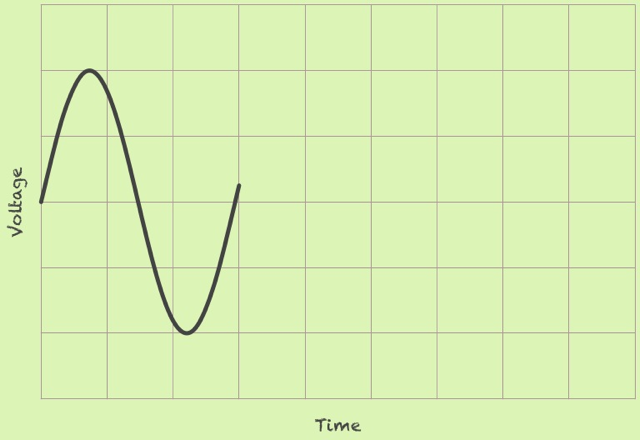
The DFT determines what frequencies are present in a signal. The algorithm is based on the idea of an infinitely long input, meaning that if your input is a single cycle of a sine wave:

 

…the DFT will actually see it as an endless repetition of that sine wave:

 

The resulting spectrum contains just a single spike at the signal’s frequency:

 

This is fine for a signal that just happens to line up nicely with sampling time. But what about a signal like the following one?

 

 

The DFT will see this as a signal that jumps straight from the maximum value to zero, repeatedly:

 

This is of course quite a different signal from a pure sine wave. You would expect its DFT to be different than the single spike we saw above, and indeed it is:

The peak gets smeared out across the frequency domain. The noise floor rises up, and may obscure other frequencies that are present in the signal. It would be nice to reduce this effect and get a cleaner spectrum.

Why Window?

Having a discontinuity in your signal is a bit like building a transcontinental railroad and discovering at the last mile that the two ends are not quite going to line up. You need to bend the tracks a bit to get them to fit.

In the world of spectrum analysis, this bending is referred to as windowing. A window function alters your signal, tapering it to nearly zero at the beginning and end:

 

 

The DFT will see an infinite number of repetitions of this new signal:

 

 

The discontinuity has been eliminated, but at a cost. You are no longer looking at the original pure sine wave. Instead, you are looking at a sine that pulses repeatedly, like an amplitude-modulated signal. The new spectrum reflects this difference:

 

 

The spectrum is not smeared out as dramatically as before, but the peak is now a bit wider. It no longer comes to quite as sharp or high of a point. Other peaks, side lobes, have arisen to the left and right.

The window function, the shape we choose for our window, determines what kind of distortions we see in the spectrum. Different window functions help you to optimize for different goals: a more accurate amplitude, a lower noise floor, and so on. In the next section, I will explore a few of the more common window functions and their uses.

Common Window Functions

Kaiser

The example window above is known as the Kaiser window. It strikes a balance among the various conflicting goals of amplitude accuracy, side lobe distance, and side lobe height.

Choosing this window will often reveal signals close to the noise floor that other windows may obscure. For this reason, many spectrum analyzers default to this window.

Hamming and Hanning

These two similarly-named Hamming and Hanning (more properly referred to as Hann) window functions both have a sinusoidal shape. The difference between them is that the Hanning window touches zero at both ends, removing any discontinuity. The Hamming window stops just shy of zero, meaning that the signal will still have a slight discontinuity.

 

Both of these windows result in a wide peak, but nice low side lobes:

 

Between the two, the Hamming window does a better job of cancelling the nearest side lobe, but a poorer job of cancelling the rest. Due to their speed and good-enough noise performance, these windows have historically seen use in voice communications.

Blackman-Harris

The Blackman-Harris window is a more elaborate version of the sinusoid approach used by the Hamming and Hanning windows.

 

The resulting spectrum has a wide peak, but good side lobe suppression:

 

This looks a lot like the Kaiser window—a fact which did not go unnoticed by Harris himself. Like Kaiser, Blackman-Harris is a decent general-purpose window.

Flat Top

The flat top window has a surprising shape. It actually crosses the zero line:

 

The result is a much broader peak in the frequency domain:

 

Crucially, this broad peak is closer to the true amplitude of the signal than with any of the other windows. The flat top window is therefore a good choice when your top priority is measuring your signal’s amplitude from the spectrum.

Rectangular

We’ve already seen the rectangular window: it’s just another word for no window at all. Technically, the term also includes windows that drop abruptly from full strength to zero (no tapering), but in practice people usually use it to mean an un-windowed signal.

Because of the spectral issues we have discussed, the rectangular window is less useful than the others as a general-purpose window. It is, however, a good choice for viewing transient signals.

Window Factor

In addition to affecting the shape of the spectrum, the window also influences acquisition time. You may recall the tradeoff between resolution bandwidth, or RBW (the instrument’s ability to tell apart signals that are close together) and number of samples. The narrower your RBW, the more samples you need.

My co-worker Alan Wolke likens this phenomenon to watching freeway traffic. The closer a car’s speed to your own, the longer you have to watch it to tell whether it’s moving faster or slower than you.

These two factors—acquisition time and RBW—are related by a simple formula:

You can think of the window factor as a measure of how pinched a window’s shape is in the time domain. With a window like Flat Top that squeezes out a lot of data, you’re going to have to acquire more samples to make up for the loss.

Window Factors (source)

Window	Factor
Kaiser	2.23
Rectangular	0.89
Hamming	1.30
Hanning	1.44
Blackman-Harris	1.90
Flat-Top	3.77

Further Exploration

One of the best ways to explore the various windows is to connect a signal to your spectrum analyzer and cycle through the choices with different input signals. In particular, see what happens when you vary the input frequency slightly. Some windows have consistently good performance for any input, while others (such as the rectangular window) vary considerably from better to worse.

Stanford University has an informative online book that introduces the various window functions. Here, you’ll find both the nuts-and-bolts mathematical definitions and a high-level discussion of the tradeoffs each window function offers.

Is there an aspect of window functions that you’ve always been curious about? Do you have a favorite window that’s not among the ones listed here? Feel free to drop me a line in the comments.