Getting Started - It is easy to use MATLAB with your Tektronix oscilloscope over a USB connection. The goal of this guide is to allow you to verify within 15 minutes that you can use MATLAB with your Tektronix series oscilloscope. MATLAB enables Tektronix oscilloscope users to acquire and analyze data, graphically visualize data, make custom measurements, generate reports, and develop automated applications.
GPIB, TCP/IP, RS-232, and USB: This guide was designed to use MATLAB with an oscilloscope over a USB connection. You can also download a Getting Started Guide for using MATLAB with your instrument with a GPIB, LAN (TCP/IP), or Serial (RS-232) connection at www.mathworks.com/tektronix/start.
System requirements for completing this guide:
- A Tektronix oscilloscope with a USB interface supporting remote instrument communication.
- MATLAB and MATLAB Instrument Control Toolbox installed on a computer.
- VISA software installed on the computer. VISA is often available as a free or low cost download from instrument manufacturers.
- Appropriate MATLAB Instrument Driver for your instrument. MATLAB instrument drivers are available at: www.mathworks.com/tektronix.
Trial of MATLAB and Instrument Control Toolbox:
If you do not already own MATLAB or MATLAB Instrument Control Toolbox, you can request trial MATLAB software at www.mathworks.com/tektronix/instrument/tryit.html.
Prepare you system
Step 1: Start Test and Measurement Tool
Start MATLAB and issue the following command to launch Test and Measurement Tool:
tmtool
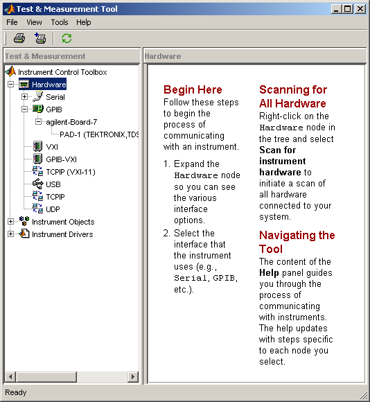
Test and Measurement Tool (Figure 1) is the graphical user interface for configuring and controlling instruments in MATLAB.
Step 2: Connect your instrument
Connect your instrument to your computer via the USB interface. Note: You will likely need to use the USB port in the back of the oscilloscope as many front USB ports do not support remote instrument control.
By default, many Tektronix oscilloscopes are already set to auto detect connections from your computer. However, you may have to enable your Tektronix oscilloscope to accept remote connections yourself. For example, select Utility > Options > Read USB Port, and ensure that the Rear USB Port is set to "Auto Detect".
Now look in the user interface for your VISA software to confirm that your PC has detected your oscilloscope. Selecting "Refresh All" or "Rescan" may be necessary to have VISA rescan for new instruments. Note the complete USB Resource name (such as USB0::1689::871::C010151::0::INSTR). You will need this Resource name in step #4.
Step 3: Locate an instrument driver
instrument drivers, which allow you to communicate with your device without knowing low-level instrument commands. To see if an instrument driver from your oscilloscope is already installed, right click on the Instrument Drivers node and select Scan for Instrument Drivers. Under the MATLAB Instrument Drivers node, look for a driver that matches your device. If you do not have a matching driver installed, check for your instrument driver at: http://www.mathworks.com/tektronix. If you are unable to find a matching driver, a driver for a similar device may work with little or no modification.
Downloaded drivers must be placed in a directory on the MATLAB path such as <matlabroot>\work. Right-click on Instrument Drivers and choose Scan for Instrument Drivers to refresh the current list of drivers.
Connect to the instrument
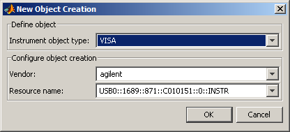
Step 4: Create the interface object
Navigate to the Interface Object node under the Instrument Objects node. Right click and select Create New Interface Object. Specify VISA, the vendor for your VISA installation, and the USB resource name. See Step 3 for instructions on obtaining the Resource Name. The resulting dialog is shown in Figure 2. Click OK to close the dialog box.
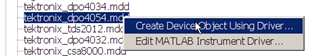
Step 5: Create the device object
Under the MATLAB Instrument Drivers node, right click on the instrument driver for your device and select Create Device Object Using Driver as in Figure 3. In this example, the instrument is a Tektronix TDS4054. In the resulting dialog box, select the interface object you created in Step 4.
Click OK to complete the creation of the device object.
Step 6: Connect to the device object
Select the newly created instrument object, which in this example is labeled scope-tektronix_tds4054, under the Device Objects node. Now click Connect in the upper right hand corner and you are ready to start interacting with your device.
Interact with the instrument
Step 7: Query a property
Select the instrument object, click on the Properties tab, navigate to the Timebase property in the group, and click Get as in Figure 4. The results appear in the Response region in the right side.
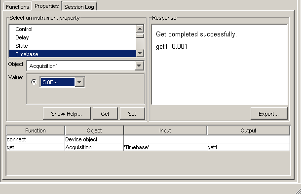
Step 8: Configure a property
Navigate to the Timebase property then choose a value for the property and click Set. The Response region indicates if the set succeeded or displays an error message indicating the reason if it failed.
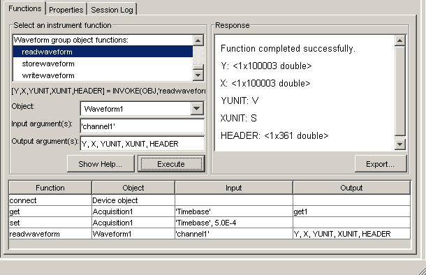
Step 9: Invoke a function
View the instrument's functions by choosing the Functions tab. To call the readwaveform function, first scroll to readwaveform under the Waveform group in the function list. Then enter input argument 'channel1' (include the single quotes) to read the first channel. Next enter output arguments Y, X, YUNIT, XUNIT as a comma separated list. Finally, click Execute to read the waveform. The results appear in Figure 5.
Step 10:Visualize results
Choose the menu item File > Export > Instrument Responses. To plot the waveform (variable Y) from the resulting dialog (Figure 6), check only the box to the left of variable name Y and uncheck all others.
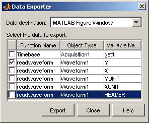
In the Data Destination drop-down, choose MATLAB Figure Window and click Export. This will create a MATLAB Figure window displaying the waveform you captured.
Step 11:Analyze results
You may further analyze your data by exporting it to the MATLAB workspace. From the Data Exporter (Figure 6), choose MATLAB Workspace as the data destination then click Export. Note: Once your values and waveforms are in the MATLAB workspace, you may use them with MATLAB functions or scripts including ones you create (not shown here).
Step 12:Reuse your session
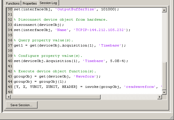
Test and Measurement Tool automatically generates MATLAB code for all of your interactions with your instrument. Select the Session Log tab of your instrument object to view the MATLAB code (Figure 7). Furthermore, using the Save Session button, you may export this code as an M-file which you can use to repeat your steps or develop a larger application.
If you have successfully completed all these steps, you have verified that you can use MATLAB and the Instrument Control Toolbox with your instrument. Additional MATLAB examples are available at: www.mathworks.com/tektronix.