How Spectrum View Outperforms Traditional Oscilloscope FFTs with Tighter Frequency Resolution Over Wider Ranges
Debugging embedded systems often involves looking for clues that are hard to discover just by looking at one domain at a time. The ability to view time and frequency domains simultaneously can enable you to measure a power rail’s voltage during wireless transmissions or observe nearfield EMI during load changes. This mixed domain analysis provides synchronized views of time domain waveforms and frequency domain spectra. For thorough high-frequency ripple analysis, it is important to make measurements over wide frequency spans with tight frequency resolution. This post explains how the 4, 5 and 6 Series MSOs enable both mixed domain analysis and wide captures with excellent frequency resolution.
Historically, to enable designers to perform frequency domain analysis, oscilloscopes have included FFTs (Fast Fourier Transforms). On power rails it is easier to understand the characteristics of noise in the frequency domain. In the time domain, noise may appear as just a fuzzy waveform, but in the frequency domain you can determine if it is broadband random noise, or perhaps crosstalk from another signal. However, FFTs are difficult to use for two reasons.
First, traditional oscilloscope-based FFTs often rely on traditional oscilloscope controls such as sample rate, record length and time/div to make adjustments to the FFT. Although it is possible to get good results using these controls, they are not intuitive. Most engineers prefer to approach frequency domain analysis using spectrum analyzer controls like center frequency, span and resolution bandwidth (RBW).
Second, even if the scope offers spectrum analyzer style controls, the FFT is driven by the same acquisition system as that used for the analog time domain view. Changing the center frequency, span or resolution bandwidth will change the scope’s horizontal scale, sample rate and record length in unanticipated and undesired ways.
To overcome challenges like these, Tektronix offers a unique analysis tool called Spectrum View in the 4, 5 and 6 Series MSOs. These instruments feature an independent signal path and digital downconverter (DDC) for spectrum analysis. This enables the use of familiar spectrum analysis controls (Center Frequency, Span and RBW) while allowing you to optimize both time domain and frequency domain displays independently. In addition to Spectrum View, the 4, 5 and 6 Series MSOs also support traditional oscilloscope FFTs in their waveform math. This will make it easy to compare Spectrum View with traditional FFT, especially for power rail noise analysis.
Let us examine the differences between a traditional oscilloscope FFT and Spectrum View by using a reference design board and probing on the DC signals on this board. For this experiment, we are using an ASUS Tinker Board S model, and probing at the 3.3V DC pins. This board includes a small power distribution network (PDN) with multiple DC rails. The setup diagram is shown in Fig 1.
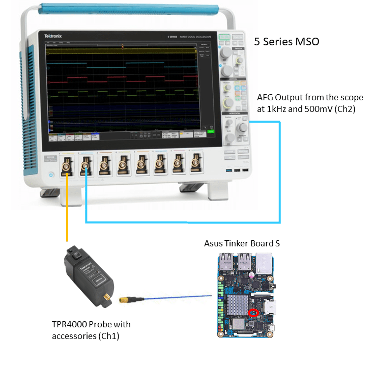
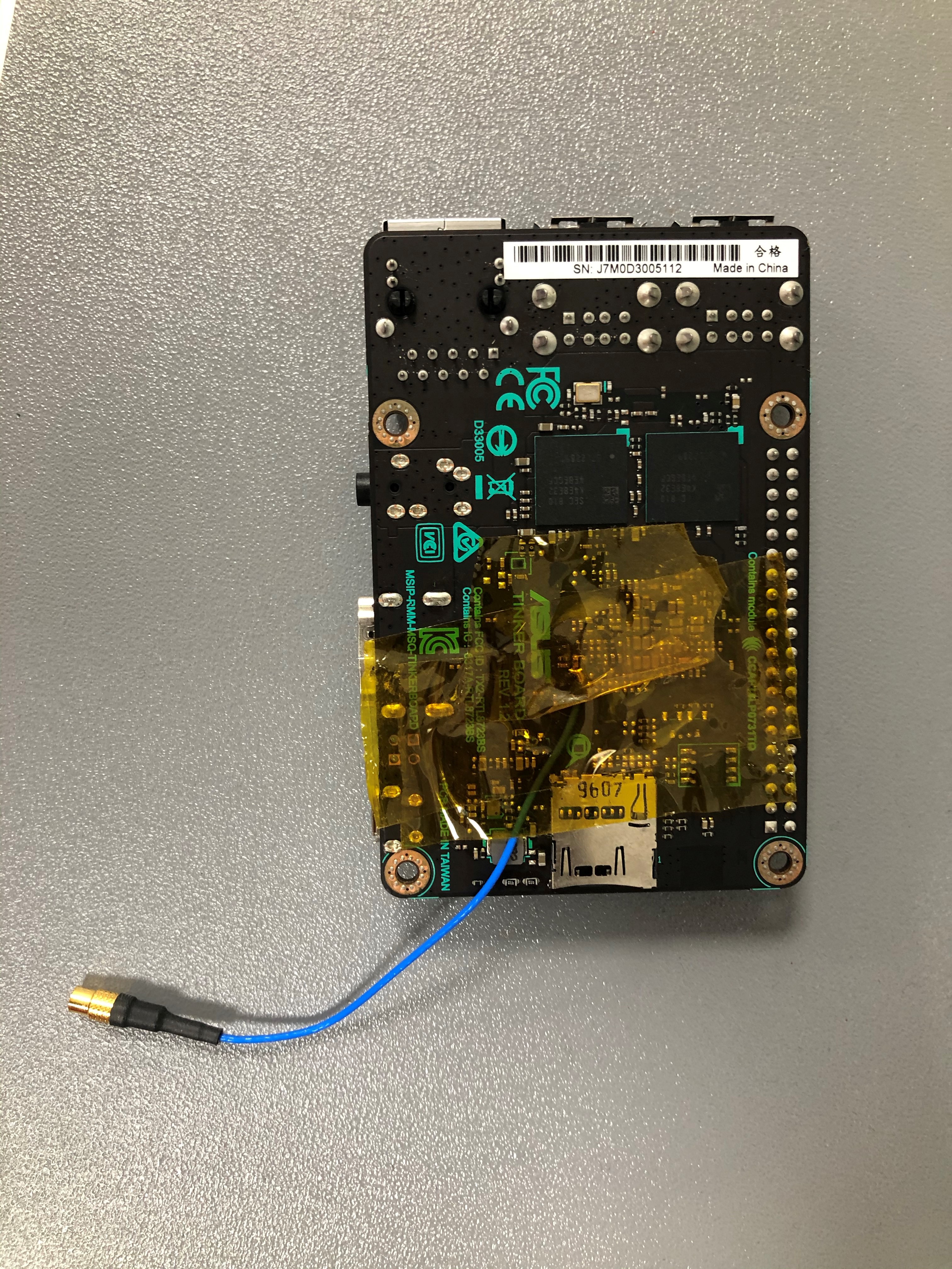
Figure 1. Setup diagram for computing FFT on the reference design board
In this case, a DC signal from the reference board is probed using a TPR1000/4000 power rail probe and connected to Channel 1 on the 5 Series MSO. This 3.3 V power rail is well within the range of this probe, with its DC offset range of +/- 60V. The probe offers a DC input resistance of 50 kΩ to reduce measurement system loading, making it an ideal probe for performing power rail measurements.
The 5 Series MSO offers an optional built-in AFG feature. Using this AFG, a 1 kHz sinewave is generated at 500 mV peak-peak and this signal is fed into Channel 2 on the scope. This will help us understand the impact of FFT on ideal sine waves and real-world DC signals.
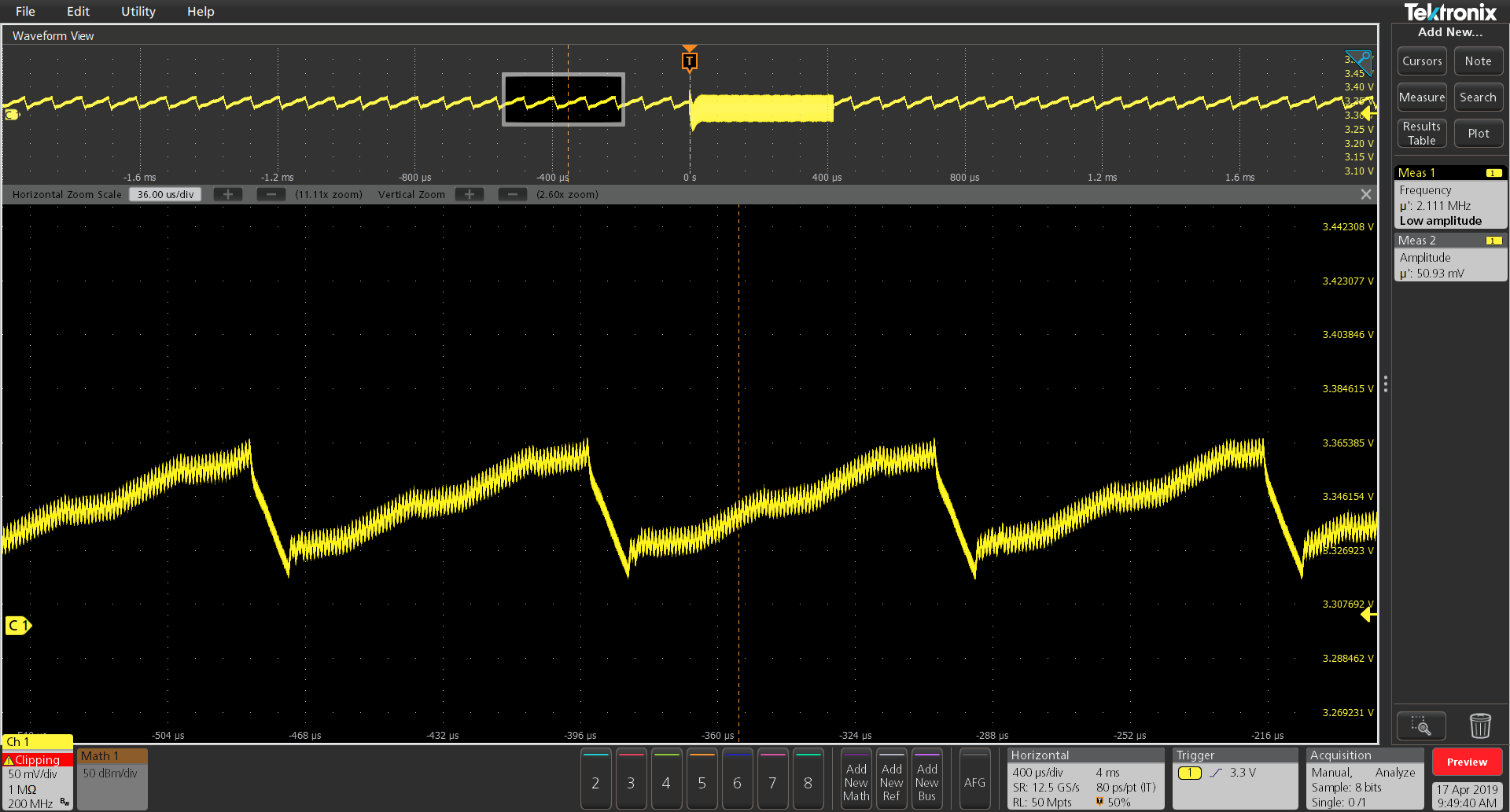
Once the signals are connected, let us enable both traditional FFT analysis using waveform math and enable Spectrum View on the same two channels. This provides us with a scope display as shown in Figure 2. Note that the 3.3V DC signal amplitude on Channel 1 varies between 3.33V and 3.38V and exhibits a ripple frequency of 3.871 kHz. This can be measured using the scope frequency measurement. Alternately, if you have multiple DC rails, you can leverage the optional 5-DPM solution which computes the RMS, frequency and peak to peak value of the ripple on up to seven DC rails on the eight channel 5 Series MSO simultaneously. This measurement is shown as the “Meas 1” badge in Figure 2.
A key feature of Spectrum View is the ability to capture and display time-correlated time and frequency-domain signals.

Figure 2. FFT using waveform math and Spectrum View enabled on both the channels with RBW = 500 Hz. Channel 1 (yellow) is connected to an actual power rail, while Channel 2 (cyan) is connected to a sinewave from a function generator.
For the first example, let’s set the Spectrum View RBW = 500 Hz. This setting uses a wider window to separate the frequencies and reports results similar to the FFT method. With this setting, let us compare the traditional FFT results with Spectrum View results.
For the power rail on Channel 1, at 3.8 kHz the FFT reports a value of -26 dBm as compared to Spectrum View which reports a value of -25.5 dBm. On Channel 2, we see an FFT value of -2.002 dBm versus Spectrum View which reports -2.303 dBm. We do not see much difference between the two methods at these settings.
Now, let us reduce the RBW window setting on the Spectrum View to 100 mHz, and observe the results as shown in Figure 3. Note that we can independently change the Spectrum View settings without altering the time-base settings in the waveform view. However, we are not able to independently change the frequency resolution on the traditional FFT without impacting record length or sample rate.

Figure 3. FFT using waveform math and Spectrum View on both the channels with RBW = 100 mHz
With the significantly lower RBW in Spectrum View, the level on our power rail at 3.8 kHz is now -44.7 dBm. Of course, the reading for the FFT has not changed and continues to report a value of -26 dBm. On Channel 2, we see an FFT value of -2.025 dBm versus Spectrum View which reports -2.02 dBm. So, for an ideal sine waveform, there is not much difference in the reported values. However, we’ve seen that this is not the case for practical power rails with ripple and noise at multiple frequencies. For the real power rail signals, Spectrum View reports more accurate test results with the ability to measure with frequency resolution which is not practical using traditional FFTs.
Table 1. Looking at power rail noise on an Asus Tinker Board 3.3V DC rail with 500 Hz resolution and 100 mHz resolution gives different results.
|
Spectrum View (dBm) |
FFT (dBm) |
RBW |
Notes |
|---|---|---|---|
|
-25.5 |
-25.917 |
500 Hz |
SR = 625 MS/s and RL = 2.5 M |
|
-44.7 |
-26.57 |
100 mHz |
SR = 625 MS/s |
If you wanted to perform a similar measurement with 100 mHz RBW with a traditional FFT you would need a record length of 12.5G samples. This is an impractical record length. This is because with traditional oscilloscope FFTs the maximum frequency of the spectrum is governed by sample rate. High sample rates consume record length quickly. The frequency resolution (or RBW) is governed by the time duration of the acquisition. Thus, for any reasonable record length, higher frequencies must be viewed with lower frequency resolution.
The digital downconverters in the 4, 5 and 6 Series MSOs break this constraint, enabling the use of small RBWs independent of center frequency in the Spectrum View.

Figure 4. Ripple of approximately 1 kHz combined with ripple on ripple of 2.1 MHz. Analysis requires wide spans and fine frequency resolution.
Power rail probes like the TPR1000 and TPR4000 Series offer bandwidth of 1 GHz and 4 GHz respectively. By combining TPR1000/4000 Series probes with Spectrum View, designers can measure very high frequency ripple values with excellent frequency resolution, which is typically not possible with conventional FFTs. This kind of high-frequency ripple is shown in Figure 4 as ripple on ripple.
For analyzing noise on power rails, key advantages of Spectrum View include:
- Enables the use of familiar spectrum analysis controls (Center Frequency, Span and RBW)
- Improves update rates and strengthens frequency resolution with hardware digital downconverters
- Allows optimization of both time domain and frequency domain displays independently
- Enables a signal to be viewed in both a waveform view and a spectrum view without splitting the signal into different inputs
- Enables accurate correlation of time domain events and frequency domain measurements (and vice versa)
- Significantly improves achievable frequency resolution in the frequency domain
For more details on analyzing power integrity on a power distribution network using power rail probes and automated measurements, visit: https://www.tek.com/application/analyzing-power-integrity-on-pdns