Real-time digital oscilloscopes are ubiquitous in today’s electronics labs. Understanding the signal processing that takes place is essential to getting the most out of these instruments. A common source of confusion is the processing that digitized samples go through from the analog-to-digital converter (ADC) to the display and measurement system.
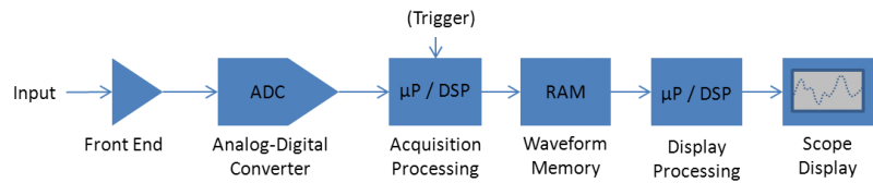
The block diagram below shows the generic flow that a signal takes from the scope’s input to the display. The analog signal conditioning in the front end, and the details of the trigger system will not be discussed in this post, but rather we’ll focus on the digital signal processing from the ADC to the display.

The front end’s job is to scale/filter the analog signal before presenting it to the input of the ADC. The ADC samples the input signal at a fixed sample interval, ts. One of the banner specifications for any digital oscilloscope is the sample rate, which is quite simply equal to 1/ts. Sample rates for the highest performing Tektronix oscilloscopes are now in excess of 100 GS/s per channel.

The amount of memory required to store a captured signal depends on two parameters: the sample rate and the time duration of the waveform. The time duration of the waveform is most often simply determined by the horizontal scale setting on the scope (what we used to call, sweep speed). The horizontal scale is given in units of time per division, such as ms/div or µs/div, etc. Since most scopes have 10 horizontal divisions, the total time duration is simply 10x the horizontal time scale. For example, if a scope uses a 5GS/s sample rate (200ps sample interval), and the horizontal scale is 20µs/div, then the waveform memory required will be 1 million points.
5GS/s x 20µs/div x 10 div = 1 million samples.

It is clear that for a given sample rate, the memory length requirements can become huge for longer time durations. The solution to this dilemma is to reduce the sample rate of the stored waveform. In general the reduced sample rate for longer duration captures is accomplished by applying some processing after the ADC, as opposed to reducing the ADC sample rate directly. There are various methods that are commonly used to reduce the sample rate to fit longer duration waveforms into waveform memory. These methods are referred to as acquisition modes.
The reduced sample rate implies a “desired” waveform sample interval. The sample acquisition mode is the default for most digital oscilloscopes, and is the simplest to understand. In this mode, one sample is saved in memory during each desired waveform sample interval as shown below, and the remaining samples are simply thrown away. The process is also called simple decimation. It is fast and easy to implement, but does result in potential loss of “interesting” samples.

The peak detect acquisition mode is used to help discover if any “interesting” sample points would be lost in the aforementioned sample mode. Here, the highest and lowest peaks from adjacent pairs of sample intervals are saved and put into memory. Thus, any abnormal high or low values, glitches, etc. will be clearly captured in the waveform memory so that further investigation of these anomalies is possible. In this mode, there isn’t any data loss, but the precise waveform shape will be somewhat obscured by the high/low value envelope.

The Hi Res acquisition mode (short for high resolution) available on Tektronix oscilloscopes reduces the sample rate on-the-fly, in-situ averaging of sample points. All of the sample points within the desired waveform sample interval are averaged together into a single point. While this acquisition mode will tend to hide glitches, and will reduce the bandwidth due to the filtering effect of the averaging, it does have the advantage of reducing noise/variation in the waveform and it improves the vertical resolution. It is also an anti-aliasing filter. For each 2x reduction in sample rate, the vertical resolution is improved by 0.5 bits. Practical considerations limit this improvement to 12-14 bits of resolution.

Each of the above modes operates on single-acquisition data. When considering multiple consecutive acquisitions, there are two additional acquisition modes:
- Average mode: This mode averages together multiple sample mode waveforms. The number of acquisitions to average together is set by the user.
- Envelope mode: This mode uses the peak mode, and builds a waveform envelope by updating the min/max values in each waveform interval with the min/max values from successive acquisitions.
Now that the waveform is stored into waveform memory, either at full sample rate or a reduced sample rate per one of the above methods, the next step is to display the waveform on the display. Modern digital oscilloscopes typically use a display which simply amounts to a flat panel LCD display. Most often, these displays have about 1000 pixels available horizontally to display the waveform. Thus, the next important question is: How is the full waveform record in memory, which can be millions of points, displayed on a screen that can only show 1000 points?

The display processing of the waveform data is responsible for accurately portraying the waveform that is in memory using the limited number of samples points in the display graticule. Most modern scopes do this by compressing the samples into the available display points in some fashion. Better scopes take all of the points that are contained in a “display point interval” and plot them all in their respective pixel columns. This results in many points being plotted “on top of each other.” The sample density or overlap of these points is typically mapped into an intensity variation of the displayed waveform color allowing the user to easily observe the typical waveform shape and the noise/uncertainty simultaneously.
As the user “zooms” the waveform, fewer points will be overlapped, until the actual samples are displayed in each pixel column. Further “zooming in” of the waveform results in waveform samples being spread across fewer display columns. In this situation, the waveform points are often connected by a graphic line that is generated by the display processor. This waveform line uses interpolation to “fill-in” the gaps between the sample points. The interpolation that is used most often is the sin(x)/x method.
It is important to understand the processing involved in creating the waveform record, as well as creating the displayed waveform, from the raw full-sample rate data. Not only can the choices made have an impact on the waveform (lost data, etc.), but it can also affect the measurements made on the waveform record. Some manufacturers, for example, may use decimated data from the waveform record, or even the display points alone, when making automated measurements. With long record length data, this will significantly speed up the processing, but it can also lead to inaccurate results due to inadequate sample density for a given measurement. Measurements made on Tektronix digital oscilloscopes always use un-decimated waveform data for automated measurements. This process can be slower for long record lengths, but it ensures accurate results that do not change with the displayed zoom level.
There is certainly a lot more to the story of how waveforms are displayed on a digital oscilloscope, including factors and topics such as display persistence, waveforms per second and interpolation details. But, hopefully this short post gave you a basic understanding of how your signals are processed onto the screen of your digital oscilloscope.