Meeting the Demands of Modern Radar Testing
In designing modern electronic warfare and radar systems, you face significant challenges. You must develop solutions with the flexibility and adaptability required for next-generation threat detection and avoidance. To succeed, you need capable tools for the generation and analysis of extremely complex pulse patterns and you need to validate designs with advanced scanning methodologies – tools that can handle complex radar baseband, IF and RF signals as well as identify multi-system interference.
With today’s rapid advances in radar technology, developing and manufacturing highly specialized and innovative electronic products to detect radar signals takes leading-edge technology and tools. Tektronix innovative radar testing equipment reduces testing uncertainty during the design process and delivers confidence in the integrity of increasingly complex designs. Tektronix Arbitrary Waveform Generators, Real-time Spectrum Analyzers and High-Bandwidth Oscilloscopes offer the capabilities you need to manage the requirements of modern radar applications. Real-time visibility of advanced pulse compression systems and the generation and analysis of all digital dynamic signal types help you create highly reliable, cost-effective system designs for defense and commercial electronic systems. The broad portfolio of Tektronix generation and analysis tools represents a scalable architecture that can protect your investments and speed your design development.
Time and Frequency Domain Analysis
Instrument Considerations
To understand the best measurement device, we need to understand the signals we are dealing with. First, we assume a sensor (Radar) or an ECM is mostly characterized as a time domain phenomenon, as fundamentally we are dealing with the transmission of a quantity of electromagnetic energy that illuminates a target - we then measure the time it takes for the reflected residual energy to arrive back at the receiver. The signal could be a continuous wave or a sequence of pulses with a specific mission goal. However, pulse rise and fall times, the type of modulation and the behavior of the transmitter amplifier and most importantly the frequency of transmission can create a broad range of responses that need to be considered.
Time domain measurements are traditionally performed with oscilloscopes while spectrum analyzers are best suited for frequency domain measurements. However, our problem is unique; in that we have time domain behaviors we want to observe, but they are exhibited in the frequency domain. While swept spectrum analyzers offer wide frequency and dynamic ranges, their ability to characterize time domain data is limited. Oscilloscopes offer excellent time domain analysis, but lack in dynamic range especially at high frequencies. Advancements however in analog to digital converter technologies and in measurement instrumentation architectures such as FFT based analyzers or Vector Signal Analyzers capturing both the phase and amplitude components of the signal, or its vector) now allow for wide instantaneous bandwidth captures of high dynamic range time domain data in the frequency domain. This is key when dealing with a transient/pulse-based time domain system with transmission frequencies in the giga-hertz ranges such as a radar or ECM.
Real Time Spectrum Analysis drives to the next level of insight. The advantage of real-time measurement capability is the ability to capture transient events in the frequency domain; real time multi-domain triggering, time-selective spectrum analysis, continuous wide bandwidth waveform storage and high-quality persistent displays that provide the higher levels of measurement capability and insight.
Signal Characteristics
As discussed, two types of signals need to be characterized,CW and Puled, with each having its own mission advantages and disadvantages.
CW Radar - Continuous-wave radar is a type of radar system where a known frequency of continuous wave radio energy is transmitted and then received from any reflecting objects. Continuous-wave (CW) radar is excellent for calculating velocity using the Doppler effect by comparing the frequency shift of the received signal with that of the transmitted. Test equipment needs to have the required broadband performance to capture the CW signal with enough fre quency resolution to analyze the Doppler frequency shift.
Pulsed Radar - A pulsed radar emits short and pow¬erful pulses and in the silent period receives the echo signals. It is excellent for determining range by measuring the time difference between the transmitted pulses and the received pulses. The Doppler effect can also be observed to measure velocity, however it is usually calculated over multiple pulses.
Both types of radar could employ various types of modulation.
Measurement Considerations
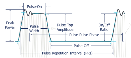
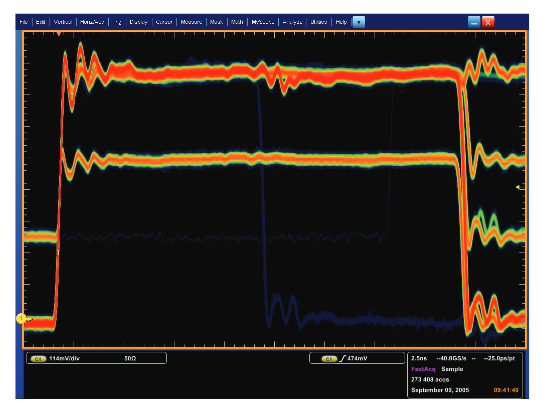
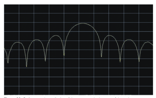
For CW radar the instrument must be able to capture the transmission frequency plus the reflected doppler shifted frequency. For pulsed radar there are two options – the first is capture the lower frequency envelope information such as PRI (Pulse Repetition Interval) using a detector, or capture all the signals information with a broadband instrument such as a wide bandwidth Oscilloscope or Spectrum Analyzer. The darker line in Figure 1 shows the time domain envelope of the pulse and the lighter lines show the sinusoidal energy that fundamental makes up the pulse.
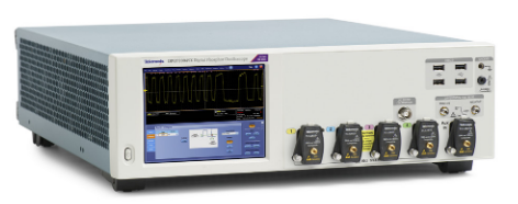
Another important factor is to ensure the instrument has enough bandwidth to capture the rise/fall times correctly. For example, an impulse radar may have a very short duration pulse therefore a very broadband oscilloscope may be the best tool to capture the pulse and characterize its parameters such as overshoot and rise and fall times. Very fast transition times or very short duration (sub-nanosecond or shorter) can be accurately seen on a 70 GHz bandwidth oscilloscope such as the DPO70000SX family.
For measuring on/off ratio a wide amplitude is required, Understanding the dynamic range of the instrument is key for this measurement, sometimes referred to the dynamic range of an instrument, ab and can be expressed in decibels, actual bits or effective number of bits (ENOB).
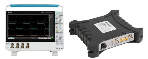
For example, the Tektronix 4, 5 and 6 Series MSO oscilloscope has a 12 Bit analog to digital converter (ADC) and can capture signals with up to 8GHz in bandwidth. The MDO4000C has an optional Spectrum Analyzer built in with an RF frequency range up to 6GHz not only does this allows for cross domain triggering but also provides higher dynamic range for frequency domain measurements The 5 and 6 Series can be used alongside a USB spectrum analyzer such as the RSA300 or RSA500 families when wider frequency coverage and better dynamic range is required, especially for frequency domain measurements.
If the pulse has vector modulation as used in data link or communication systems, this may require specialized demodulation measurements such as error vector magnitude (EVM). Advanced frequency and vector analysis is provided the SignalVu PC that can connect to both Oscilloscopes and Spectrum Analyzers.
Oscilloscope Measurements
The oscilloscope is the fundamental tool for examining varying voltage versus time. It is very well-suited for displaying the shape of baseband pulses. The origin of oscilloscope performance parameters traces back to characterizations of early radar pulses. Today’s real-time oscilloscopes have bandwidth up to 70 GHz, and are designed to capture and display either repetitive or one-shot signals.
Modern Oscilloscope triggering systems are very highly developed and can trigger on both analog and multiple channels of digital data. For example the 5 series oscilloscopes eight input channels can be assigned as trigger inputs for both analog signals such as the envelope of an individual pulse, a defined stream of pulse envelopes or each channel can be assigned to a further eight digital inputs, providing the capability to trigger on multiple parallel data lines or words. Utilizing the external trigger RF devices such as the RSA300 or RSA500 families of spectrum analyzers can be triggered to perform frequency domain measurements based on real-time analog or digital domain events.
Pulse Measurements
The FastAcq feature of the oscilloscope operates on live time-domain data using DPX™ acquisition technology. All frequency domain measurements are made on the timesampled acquisitions of stored data.
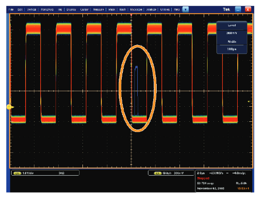
The FastAcq display on the oscilloscope can discover baseband pulse time-domain transient errors. Figure 4 shows just one single pulse that has a narrower pulse width than even hundreds of thousands of correct pulses. The blue color on the temperature scale representation of signal persistency represents the least frequent occurrence, while the red areas are the parts of the signal that are the same every time.
The FastAcq capability on the DPO, DSA, and MSO Series provides a time-domain display with a high waveform capture rate. The DPX acquisition technology processor operates directly on the digital samples live from the A/D converter.It discovers rapid variations or one-shot events in the timedomain display.
For wideband measurements using an oscilloscope, FastAcq can be used to see even momentary transient events using the voltage vs. time display.
Figure 5 shows a one-time transient in blue. For this display,blue represents very low-occurrence transients, while red represents parts of the waveform that are constantly recurring.
Oscilloscope Triggering
One of the most highly developed capabilities of the oscilloscope is triggering. Recent advances in oscilloscope trigger have enabled methods of triggering an acquisition or measurement based on the voltages and voltage changes in one or more channels.
These range in complexity from simple edge or voltagelevel triggering to complex logic and timing comparisons for combinations of all of the input channels available. Pattern recognition, both parallel and serial, triggering on “runt” or “glitch” signals and even triggering based on commercial digital communications standards are all available in oscilloscopes.
The 5 and 6 Series MSO, DPO7000 and DPO/MSO/DSA70000 Series oscilloscopes allow the user to specify two discrete trigger events as a condition for acquisition. This is known as a trigger sequence, or Pinpoint™ triggering. The main or “A” trigger responds to a set of qualifications that may range from a simple edge transition to a complex logic combination on multiple inputs. Then an edge-driven “B Delayed” trigger can be specified to occur after a delay expressed in time for events.
The B-trigger is not limited to edge triggering. Instead, the oscilloscope allows the B-trigger to look, after its delay period, for a condition chosen from the same broad list of trigger types used in the A-trigger. A designer can now use the B-trigger to look for a suspected transient, for example, occurring hundreds of nanoseconds after an A-trigger has defined the beginning of an operational cycle. Because the B-trigger offers the full range of triggering choices, the engineer can specify, for instance, the pulse width of the transient they want to find. Over 1,400 possible trigger combinations can be qualified with Pinpoint triggering. Sequences can also include a separate horizontal delay after the A-trigger event to position the acquisition window in time.
The Reset Trigger function makes B-triggering even more efficient. If the B-event fails to occur, the oscilloscope, rather than waiting endlessly, resets the trigger after a specified time or number of cycles. In so doing it rearms the A-trigger to look for a new A-event, sparing the user the need to monitor and manually reset the instrument.
The system can detect transient glitches less than 200 ps wide. Advanced trigger types, such as pulse width trigger, can be used to capture and examine specific RF pulses in a series of pulses that vary in time or in amplitude. Trigger jitter – a crucial factor in achieving repeatable measurements – is less than 1 trillionth of a second (1 ps) rms.
For baseband pulses, the triggers based on edges, levels,pulse width, and transition times are of the most interest. If triggering based on events related to different frequencies is needed, then the RSA Series spectrum analyzer is required.
Manual Timing Methods
Traditional measurements of pulses were once made by visual examination of the display on an oscilloscope. This is accomplished by viewing the shape of a baseband pulse. The measurements available using this method were timing and voltage amplitude. These measurements were sufficient, as pulses were generally very simple.
The baseband pulses were used to modulate the power output of the radar transmitter. If it was necessary to measure the RF-modulated pulses from the transmitter, then a simple diode detector was often used to rectify the RF signal and provide a reproduction of its baseband timing and amplitude for the oscilloscope to display. Generally, the oscilloscope did not have sufficient bandwidth to be able to directly display the RF-modulated pulses, and if it did, the pulses were difficult to clearly see, and was even more difficult to reliably generate a trigger.
For these baseband pulse measurements, the measurement technique first used was to visually note the position onscreen of the important portions of the pulse and count the number of on-screen divisions between one part of the pulse and another. This is a totally manual procedure performed by the oscilloscope operator and as such was subject to errors.
Automated Oscilloscope Timing Measurements
With the advent of Analog-to-Digital converters, the process of finding the position on-screen became one of directly measuring the time and voltage at various portions of the pulse.
Now there are fully automated baseband pulse timing measurements available in modern oscilloscopes. Singlebutton selection of rise time, fall time, pulse width, and others are common. However, most of these measurements do not focus on the measurement envelopes of modulated radar signals.
When used on pulse-modulated carriers, these measurements are of limited utility, because they are presented with the carrier of the signal instead of the detected pulse. This results in pulse width measurements that are made on a single carrier cycle, and rise times of the carrier instead of the modulated pulse. Detectors may be used on the input of the oscilloscope to remove the carrier and overcome this.
When choosing the correct tool, most engineers us an oscilloscopes when performing time domain measurements, but spectrum analyzers are best suited for frequency domain measurements. As discussed earlier, radar and EW is unique, in that time domain behavior is exhibited in both the time and frequency domain. A swept spectrum analyzer offers wide frequency and dynamic ranges, but its ability to characterize time domain data is limited. Oscilloscopes offer excellent time domain analysis and trigger capability, but lack in dynamic range, especially at high frequencies.
Advancements in analog to digital converter technologies and in measurement instrumentation architectures such as FFT based analyzers or Vector Signal Analyzers (the instrument capture both the phase and amplitude components of the signal, or its vector), now allow for wide instantaneous bandwidth captures of high dynamic range time domain data in the frequency domain. This is key when dealing with a transient/pulse-based time domain system with transmission frequencies in the giga-hertz ranges such as a radar or ECM.
Real Time Spectrum Analysis drives to the next level of insight.The advantage of real-time measurement capability is the ability to capture transient events in the frequency domain; real time multi-domain triggering.
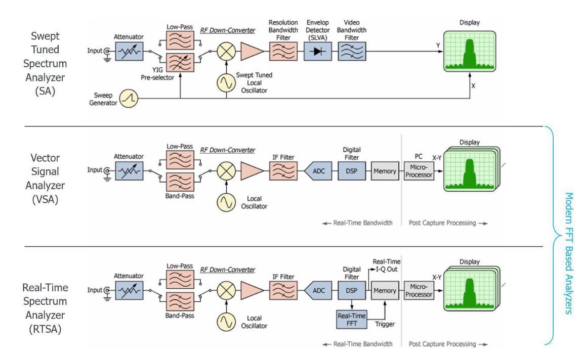
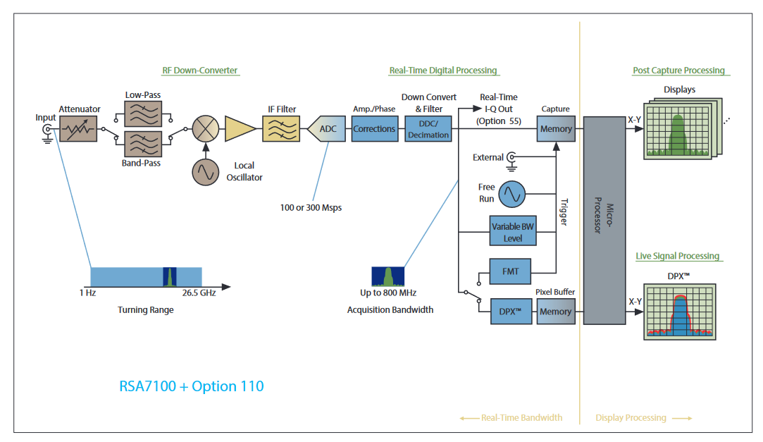
Figure 7 puts it all into context. All architecture use a super heterodyne process to convert high frequency signals to a lower frequency for analysis. The swept spectrum analyzer essential only measures the power in a filter (Resolution Bandwidth Filter) at a specific frequency point derived from the frequency of the Local Oscillator (LO). It can display a range of power vs frequency by ‘sweeping’ the LO and the x-axis of display. This allows for very broad frequency displays with excellent dynamic range, but the time domain acquisition bandwidth is limited to that of the resolution bandwidth filter. A Vector Signal Analyzer uses a fixed local oscillator, with a much larger IF filter (instead of the RBW filter bank). This allows us to acquire large amounts of time domain data,then either display it as time domain data translate it to the frequency domain utilizing an Fast Fourier Transform. A Real Time Spectrum Analyzer conceptual is the same as a VSA, however more processing is performed earlier in the signal chain allowing for faster processing of FFT’s and triggers thus providing the enhanced measurement capability required for a successful test.
What this all means is that the RTSA architecture allows us to observing time varying behaviors in the Electromagnetic Spectrum, analysis in the time and frequency domain the systems under test behavior, while simultaneously recording the events to a hard disk array.
Observing Time Varying Behaviors in the Frequency Domain
As the RTSA architecture acquires many time domain records and converts them to frequency in real time, we can simultaneously observe time and frequency. One way to display this is with a spectrogram. A spectrogram adds the dimension of time while still allowing you to observe frequency and amplitude. The x axis represents frequency, the y axis represents time and amplitude is represented by color. Usually red for high power and green for low power.
An alternate method is to visualize this measurement by emulating the anomalies of a cathode ray tube (CRT) common as the display on a spectrum analyzer before the turn of the century. A CRT utilizes a magnetically-controlled electron gun that fires electrons on a phosphor-coated screen. The screen illuminates and then slowly decays over time.
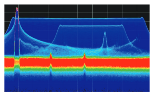
Figures 9 and 10 show a typical display using a phosphor emulation technique. Without phosphor emulation, the screen in Figure 10 would just show the large LFM signal, with the CW signal “popping out” the top on the left. But with phosphor emulation, you can see a second lower power LFM overlapped in frequency. In addition, several single-frequency pulsed carriers and two continuous wave (CW) interferers can be observed. Of course, the bandwidth and acquisition speeds are much fast than a turn of the century spectrum analyzer.
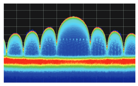
DPX™ Live RF Spectrum Display
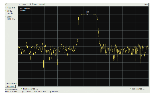
The RSA Series enables DPX™ Live RF spectrum display on up to 800 MHz acquisition bandwidth. The name DPX comes from the concept of a “Digital Phosphor Technology” display, which re-creates the slow-fade memory effect of a CRT phosphor. For the RSA, the hardware processor performs up to 292,969 FFTs per second. This gives continuous real-time visibility of varying RF signals without interruption. Figure 9 is a radar pulse with an interfering carrier sweeping through the pulsed spectrum.
The continuous non-interrupted visibility guarantees 100% probability of intercept of signals or transients as short as 3.7 μs because there is no dead time. The DPX spectrum display is observing all the time.
Interference to radar pulses and situations of multiple signals on the same frequency can all be discovered. As mentioned earlier, figure 10 is a DPX spectrum display of a chirp that has a second lower power chirp overlapped in frequency as well as several single-frequency pulsed carriers and two Continuous Wave (CW) interferers.
Automated measurements on an RSA
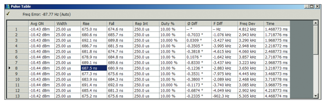
While the RSA Series can be used in a manner similar to the swept spectrum analyzer to measure in either the frequency domain or the time domain, automated pulse measurements are available that offer much more signal detail and measurement repeatability. The Advanced Signal Analysis suite, Option 20, includes the pulse measurement capability. For this analysis, the analyzer stores a digital acquisition, finds the pulses within it and measures a full set of parameters for each pulse. Timing, frequency and phase parameters are all measured. Any selected set of these parameters can be displayed or exported.
These measurement results can be further processed to display trends and analyze these trends.
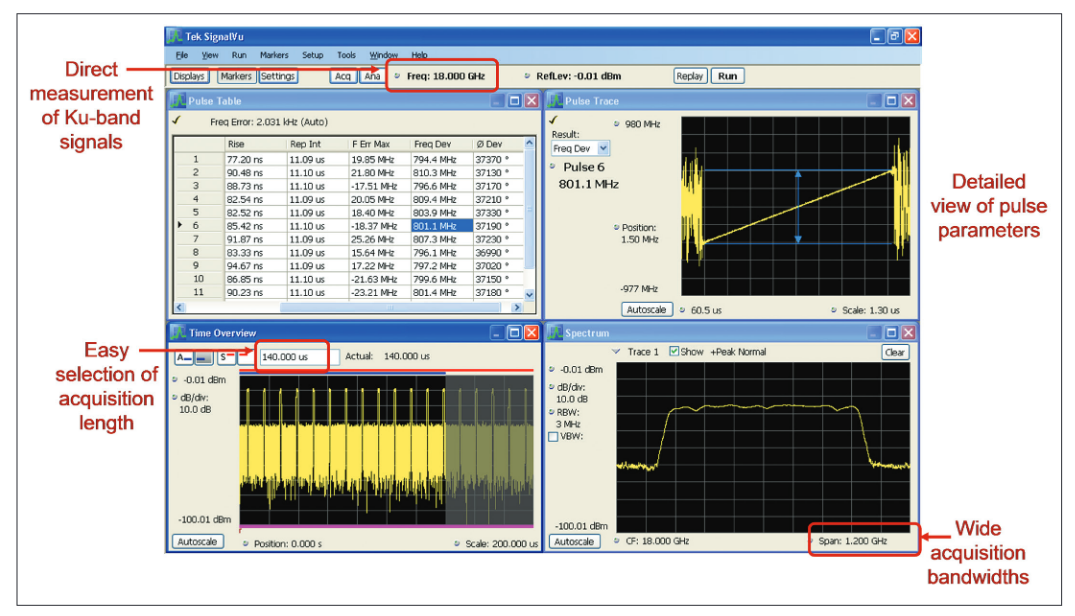
The RSA Series pulse measurement suite provides a comprehensive set of pulse parameter measurements for up to 800 MHz bandwidth, including readouts of timing,distortions, amplitude, frequency, phase and pulse time.
Some of the measurements are specifically for chirped pulses, including Frequency Deviation, Frequency Error, Phase Deviation and Phase Error. Any of the parameters with a numeric result can also have these results plotted versus pulse number, giving visibility of time-trends of errors. And lastly, these trends can be input to an FFT to determine if the errors have a coherent frequency of error variation, possibly leading to discovery of the cause of the variation.
Any or all of the measurements with numeric results can be included in the pulse table display as seen in Figure 9.
The automated pulse measurements operate on a record of data captured in a bandwidth selectable up to a 800 MHz,which is tunable anywhere up to to the 26.5 GHz RF coverage for the RSA7100
Related Measurements
he SignalVu vector signal analysis software that includes Option SVP - Advanced Signal Analysis has the same automated pulse measurement functionality of the RSA Series. It can be installed on DPO/MSO5000, DPO7000 and DPO/DSA/MSO70000 Series oscilloscopes. This combines the extremely wide bandwidth available from, for example, the DPO70000 Series at 33 GHz, with the spectrum analysis and fully automated Pulse Measurement Suite from the RSA Series spectrum analyzers.
When installed on an oscilloscope, the internal software limits on setting frequency coverage, bandwidth, and record length automatically adjust to use the frequency and memory limits of the oscilloscope on which it is installed. The SignalVu vector signal analysis software provides control of the oscilloscope attenuator, gain, sampling rate and sweep rate controls by allowing the user to control “Reference Level,” “Frequency Span” in a manner with which spectrum analyzer users are familiar.
The vector signal analysis software can use any of the input channels of the oscilloscope. It can also use the oscilloscope’s “math trace” capability to combine data from multiple channels and use math functions on the data.
he measurements will have the same dynamic range as the oscilloscope, while maintaining its full bandwidth. Figure 10 shows a span of 1.25 GHz, and a chirped pulse that is 1 GHz wide. The frequency span capability is limited only by the bandwidth capability of the oscilloscope on which the software is installed.
Just like the RSA, the pulse measurements are performed on data in the acquisition memory on a continuous capture/ analyze cycle, or on waveforms stored on the instrument hard disk drive.
| Instrument Series | Frequency Range | Bandwidth | Rise Time (20%/80%) / Min Pulse Width Detection | 3rd Order Intermodulation Distortion (typical) |
| Spectrum Analyzers | ||||
| RSA5000 | 1 Hz to 26.5 GHz | 25 MHz std; 40 MHz opt 85 MHz 110 MHz |
40 ns/120 ns 25 ns/120 ns 12 ns/50 ns 10 ns/50 ns |
<-84 dBc @ 2 GHz |
| RSA7100A | 16 kHz to 14.2/26.5 GHz | 320 MHz std; 800 MHz opt. |
-85 dBc @ 100MHz to 3.4GHz -65 dBc @ 3.4GHz to 6GHz -80 dBc @ 6GHz to 26.5GHz |
|
| Oscilloscopes | ||||
| DPO7000 | DC to 3.5 GHz | 500 MHz 1 GHz 2.5 GHz 3.5 GHz |
310 ps/16 ns 200 ps/8 ns 100 ps/3 ns 95 ps/2.25 n |
-40 dBc @ 2 GHz |
| DSA/DPO/MSO70000 | DC to 33 GHz | 4 GHz 6 GHz 8 GHz 12.5 GHz 16 GHz 20 GHz 25GHz 33 GHz |
65 ps/2 ns 43 ps/1.3 ns 33 ps/1 ns 23 ps/640 ps 21 ps/500 ps 17 ps/400 ps 17 ps/400 ps 17 ps/400 ps |
-55 dBc @ 2 GHz -48 dBc @ 10 GHz -50 dBc @ 18 GHz |
Table 2. Measurement equipment overview.
Measurement Equipment Selection Chart
The measurement tasks and the pulse parameters that are important for each task have been presented, as well as the capabilities and limitations of the various test equipment.Table 2 summarizes the test instrument choices based on the measurement characteristics needed.
Example Measurements with Radar Test Equipment
Instrument Operations
Whether using an oscilloscope or a Real-time Spectrum Analyzer, there are some controls providing flexibility of operation which may need to be set differently from the default to allow proper signal acquisition and pulse measurements. Usually it becomes necessary to adjust these only when operating outside of one or more “default” instrument settings. Measurement results can be affected by adjusting these advanced settings.
The more common of these include: Delay after Trigger (delays the start of acquisition after a trigger has been recognized); Acquisition Time and Acquisition sample length (normally these are automatically coupled to settings of Span, Bandwidth, and type of measurement in use); Units of Volts, Watts or dB (the default is dB, but some tasks may require alternate units to be selected); Alignments (the internal alignment routines may be disabled if needed for a measurement for which interruption due to internal alignment procedures would be unacceptable).
The time-domain displays (Frequency, Phase, and Amplitude versus Time) have an additional measurementilter whose bandwidth can be adjusted.
All the measurements made in the RSA5000 and RSA7100 rely on getting signals which have passed through an IF frequency converter system. For the 110 MHz bandwidth option of the RSA5000 and RSA7100, the IF filter is approximately 120 MHz wide.
Due to the nature of frequency conversion schemes that are this wide, the filter used must have relatively sharp frequency response roll-off at the filter edges. For pulses this may cause as much as 40% overshoot. For the purposes of pulse measurements there is a need for a Gaussian response filter to minimize this overshoot on a pulse. This Gaussian filter can be added to flatten pulse response at the expense of bandwidth. A non-Gaussian filter can also be selected if narrower but flat response is desired.
For the RSA hardware, there are some hardware controls to be considered, including: Internal/External frequency reference, used for locking the frequency reference so that the analyzer measures frequency referred to the external system reference; external gain or loss, used to account for an attenuator which may be used to lower transmitter power to the limits of the RSA hardware; and attenuator limits which prevent the internal attenuator from being set to zero, thereby protecting the analyzer’s front-end mixer from damage by large signals.
For the SignalVu vector signal analysis software, some of the oscilloscope controls may interact with the software controls or settings. While the default setting locks the oscilloscope controls to the analysis software settings, it is possible to override this setting and manually set sample rate, input attenuation, etc. This will cause the software to change span, RBW, and Reference Level to accommodate the manual oscilloscope settings.
The difference between Amplitude vs. Time and Time Overview
At first glance, it would appear that these two displays might well be the same thing. They are not.
The Time Overview is a very simple magnitude display which has as its source all of the decimated I/Q sample pairs of the acquisition. It is here that the subset of the full acquisition intended to be analyzed can be seen and adjusted. The portion of the acquisition that is used to create the Spectrum Display is also shown, and can be separately adjusted.
The amplitude vs. time display is one of the analyses which use the “analysis” subset of the acquisition record. This display is equivalent to the “zero-span” setting in the traditional swept analyzer. This display has its own “Time Domain Bandwidth”filter which can be used to reduce the bandwidth of this measurement for noise reduction or glitch reduction.
The Trace Decimation Control
Another one of these lesser-used controls is the “Trace Decimation” setting. Particularly for the “parameter vs. time” displays, the acquisition record being analyzed can be very large. It can be as large as the entire acquisition memory, as compared to the “Pulse Trace” which can have only the samples for one pulse. When there are several million or more acquisition samples, the trace processing may become slow. This usually happens when the digitizing rate is very high at the same time as the acquisition record length is set very long.
The trace processor has a user-selected Trace Decimation that will set a limit on the number of resulting trace points allowed in these “parameter vs. time” displays, providing faster display results.
At first glance, it would appear that these two displays might well be the same thing. They are not.
The Time Overview is a very simple magnitude display which has as its source all of the decimated I/Q sample pairs of the acquisition. It is here that the subset of the full acquisition intended to be analyzed can be seen and adjusted. The portion of the acquisition that is used to create the Spectrum Display is also shown, and can be separately adjusted.
The amplitude vs. time display is one of the analyses which use the “analysis” subset of the acquisition record. This display is equivalent to the “zero-span” setting in the traditional swept analyzer. This display has its own “Time Domain Bandwidth” filter which can be used to reduce the bandwidth of this measurement for noise reduction or glitch reduction.
The Trace Decimation Control
Another one of these lesser-used controls is the “Trace Decimation” setting. Particularly for the “parameter vs. time” displays, the acquisition record being analyzed can be very large. It can be as large as the entire acquisition memory, as compared to the “Pulse Trace” which can have only the samples for one pulse. When there are several million or more acquisition samples, the trace processing may become slow. This usually happens when the digitizing rate is very high at the same time as the acquisition record length is set very long.
The trace processor has a user-selected Trace Decimation that will set a limit on the number of resulting trace points allowed in these “parameter vs. time” displays, providing faster display results.
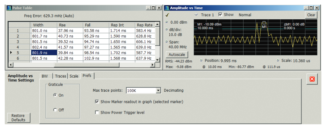
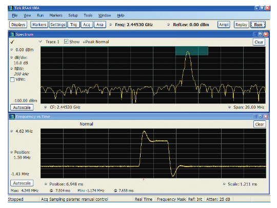
In most cases, 100,000 points should be plenty. But in the case of a radar pulse with very small duty cycle, there may be a need to zoom in on the display much more than normal. In Figure 11, the acquisition was 18.722 ms long, and has 936,112 samples taken at 40 MHz sample rate. These acquisition parameters can be found in the acquisition control tab. The maximum trace points are decimated down to 100,000 as seen in Figure 11. But to see just one pulse in the amplitude vs. time display in the upper right of the screen, the display has been zoomed to 10.36 µs wide to see just one pulse. This provides only 10.36/18722 * 100,000 = 55 points for the display. As can be seen here, 55 points is not enough to clearly see the character of the pulse.
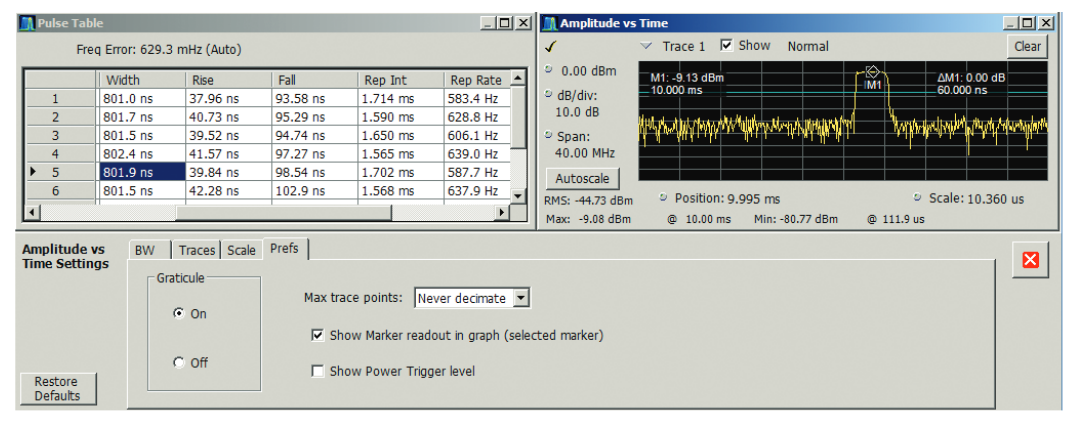
The solution is to remove the limit on trace points as seen in the lower middle of Figure 12. Now the full set of samples (936,122) of the digitized record is available for the un-zoomed trace, providing 10.36/18722 * 936,122 = 405 points in the on-screen zoomed display.
Now the amplitude vs. time trace has enough points to show the true character of the digitized pulse, visible in the upper right of Figure 12.
The number of points in the trace may not be the same as the points that are seen on-screen. The LCD screen is only capable of normal personal computer display resolution (in this case 1,024 points horizontally). If the chosen display has more points than can be displayed on the LCD, the trace must be further compressed for the display. This is done by the Windows operating system. In Figures 11 and 12, the trace has only 40% of the full screen size, or 410 pixels. Therefore, in this case the computer display has not needed to further compress the 405-point trace. There would be considerable compression of the 100,000 points if the trace were displayed without zoom.
Even when the on-screen display is further compressed by Windows, measurement accuracies are not affected. The markers and other measurements operate on the full “trace resolution.” The full-resolution traces can also be exported for further analysis or record keeping.
Characterizing Intended Radar Signals
Monitoring the intended signals emanating from a radar system may be necessary to assure compliance with regulations as well as to confirm interoperability when multiple systems are installed in close proximity to each other.
Monitoring Example: Weather Radar using RSA Series
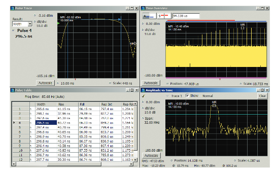
After understanding the importance of signal acquisition and trace decimation, this example demonstrated how we use time overview and amplitude versus time measurements to isolate the pulses measurements to be made. This example is a set of observations of a weather radar at 9.6 GHz. This radar is pulsed, and has a rotating antenna scanning the full 360 degrees. With several of the measurement windows separately displayed, the markers in all simultaneous windows are correlated across the multiple displays.
For a ground-based monitoring position, the measured power of the pulses will vary as the transmit antenna swings across the monitor receiver antenna.
Here the Time Overview window shows the pulses and their amplitude changes as the antenna sweeps across the monitor antenna. The marker has been placed on the highest amplitude pulse which corresponds to the time when the transmit antenna was pointing directly at the monitor antenna.
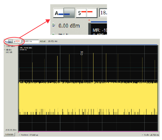
Figure 13, the four small boxes near the upper left of the display with the letter A in one pair (for Analysis) and the letter S in the other pair (for Spectrum) select the entries for the programming of the portion of the acquisition record over
which the pulse Analysis and the Spectrum analysis will be respectively performed. Which pulses out of the total acquisition record contribute to each of these sets of measurements can be separately selected.
The blue bar on the top of the Time Overview measurement indicates the Analysis Time. Note that the Analysis Length and Offset (the 2 blue buttons) will apply to all displays on the instrument except the Spectrum Display. The Spectrum Length and Offset can be set with the red buttons. The minimum Spectrum Length setting will be automatically determined by the amount of samples necessary to realize the requested RBW setting when in Auto mode. For example, narrow RBW filter will require a longer Spectrum Time. The Spectrum Length and Offset are indicated by the red bar at the top of the plot.
The amplitude vs. time trace window can be set to analyze any part or all of the acquired record. This display is the equivalent of the zero-span mode in swept spectrum analyzers. Since this particular acquisition is long enough to assure capturing the full antenna rotation across our position, there is quite a lot of data. The trace decimation may need to be disabled if zoom is needed.
The marker seen here is time-correlated with the one in the Time Overview window. This means that if either marker is moved, the other one will move to exactly the same time position. This allows measurements of different parameters to correlate all at exactly the same time.
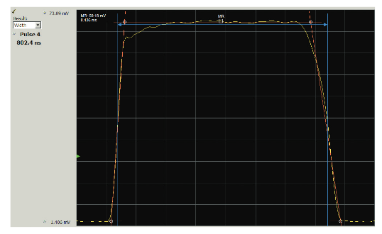
Pulse Trace is selected as the display in Figure 16 and Width is entered as the parameter to display. The readout says pulse number four is displayed. This selection will be made in the next window. For this display, the units were changed from dB to Volts. This gives a linear display and now the pulse lines and cardinal points are displayed. They are disabled whenever the display has a non-linear scale, as the lines would also go non-linear.
This is a real off-the-air radar measurement, so the antenna used and some local objects may have an impact on pulse the distortions seen here.
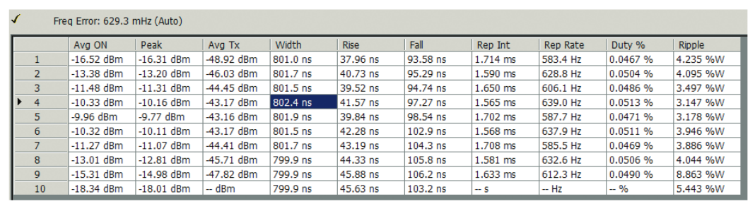
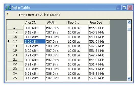
Now that the pulses are found, a table can show all of the parameters to be reported, as seen in Figure 15. Note the one cell is dark blue. When the mouse is clicked in any results cell it will become blue to signify that it has been selected, and the pulse trace window will configure itself and graphically display that particular pulse parameter. If the parameter being examined in the Pulse Trace window is changed in that window, the blue highlight selection in the Pulse Table moves accordingly
This particular weather radar radar has two modes with different pulse widths. The next pulse examined is the 300 ns pulse width in Figure 17.
When there is a need to verify many pulse measurements at once, the Pulse Measurement Suite gives rapid and complete answers.
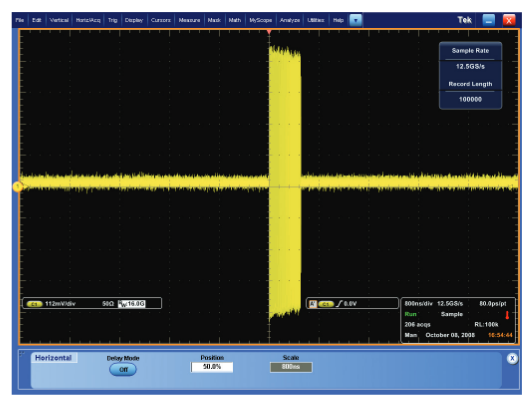
Troubleshooting Incidental Modulation Example: Wideband chirp using a DPO7000 Series oscilloscope and SignalVu
This is an example of using the SignalVu vector signal analysis software on an oscilloscope to measure a radar signal with errors in the transmitted signal. It is a chirped pulse with chirp width of about 500 MHz, which requires the greater bandwidth of the oscilloscope.
A simple view of the modulated pulse waveform is seen in Figure 18.
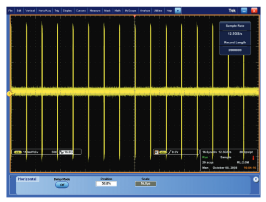
With multiple pulses included in one waveform, it is not easy to see differences between the individual pulses. If there are differences, they are more subtle than can be seen from a voltage waveform.
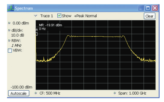
The SignalVu vector signal analysis software uses the digitized voltage waveform stored in the oscilloscope and uses the same software as the RSA Series to make all of the RF measurements. The frequency spectrum is shown in Figure 20. This pulse chirps from 250 MHz to 750 MHz.
Next the Pulse Table is selected with basic timing and amplitude measurements.
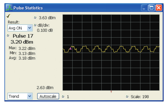
The Average ON power of the pulse numbers have very small variations showing. But they do not appear at first glance to be significant. The graphical plot of the numerical results will be more indicative if there is in fact a coherent variation. Figure 22 shows the Trend Plot of the Avg ON parameter.
To be able to see the small variations, the vertical scale has been “zoomed” to a sensitivity of 0.1 dB per division. At this setting there is very clearly a periodic variation of the pulse amplitude. The total peak-to-peak amplitude variation is about 0.07 dB.
The horizontal scale is simply the number of the pulse whose amplitude is plotted vertically. The effective way to fully analyze the variation is to use the FFT of the trend data from this plot.
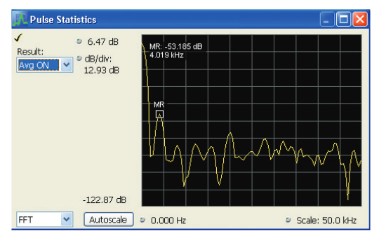
Selecting “FFT” instead of “Trend” in the drop-down box in the lower left of Figure 23 brings up the frequency spectrum of the measured parameter. The spectrum plot distinctly shows a peak disturbance at 4 kHz, which is 53 dB below the average value of the amplitude. Something is modulating the pulse power at a 4 kHz rate. The frequency of the disturbance can assist in the troubleshooting of components or subsystems within the radar causing this problem.
To convert this dB reading to the amplitude variation, work backwards through the decibel formula: V = antilog (dB/20).Minus 53 dB equates to an RMS voltage variation of 0.22%.This is 0.63% peak-to-peak. This agrees very closely with the “eyeball” value seen in the previous Figure 22.
A very subtle disturbance of this radar transmitter has proven easy to analyze.
Detecting Unintended Signals in Radar Tests
When examining an installed radar system, one important task is to check for emissions that do not help the radar and very well may cause interference. The use for radars must consider spectrum allocations as well as other nearby RF equipment and facilities. Unintended signals may also provide increased visibility of radar, or an unwanted signature which can be used to identify the radar.
Spurious
There may be signals radiated from a radar system that will create interference to other systems. These may be at frequencies outside the assigned channel of the main radar transmitter signal. Some of these signals may be active all the time and some may be active only during pulse transmission. This requires stepping across the entire frequency range of the analyzer. The wideband oscilloscope with an FFT spectrum plot can provide a single view of both in-channel and out-ofchannel emissions.
Transient Signals (DPX Live RF Spectrum Display)
Some signals may only be present during the pulse, but be on a different frequency. Some signals may be completely unrelated to the pulse, and may be on any frequency including within the pulse frequency itself.
To discover signals such as these, a monitor is needed which is continuous and also one that can show a single signal deviation out of the continuous examination.
The DPX Live RF Spectrum Display can do exactly that. This technology is implemented in the RSA hardware, so it can not be used by the SignalVu vector signal analysis software on stored acquisition records. The DPO/DSA/MSO Series oscilloscopes also utilize DPX technology for voltage vs.time traces.
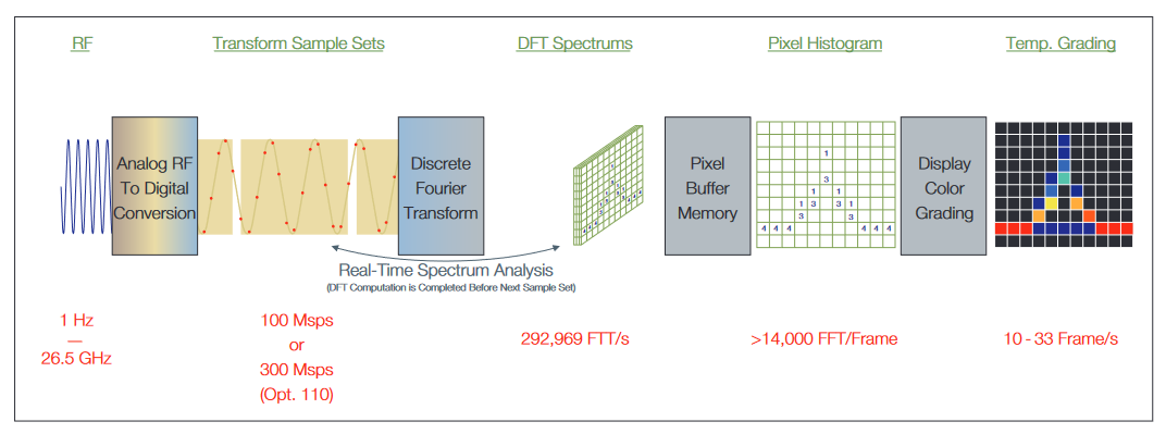
Refer to the previous Figure 5 for the RSA block diagram.The A/D converter operates continuously. Samples of whatever signal is in the IF are passed to the hardware signal processor without interruption. These samples are processed at up to 292,969 seamless spectrum measurements per second.
These spectrum measurements are done in the DPX runtime engine. The next step uses a small buffer memory (virtual screen) into which a bitmap of the spectrum display is placed. Then as each spectrum display is produced, another bitmap is added to the pixel buffer, one pixel at a time. This creates a bitmap in which each pixel contains a single number representing the number of times that the spectrum trace “hit” that location on the virtual screen.
Once the main display monitor is ready to accept the next update, the buffer pixels are converted to the different colors that represent the density of hits – blue for very few hits up to red representing many hits. In this fashion the DPX spectrum display information is updated to the display monitor without missing the presence of even one of the 48,000 spectrum measurements per second.
One last step is for the DPX spectrum display processor to check the user entry for “persistence.” If the persistence is set to minimum, then the pixel memory will be zeroed out before the next set of spectra is entered. If the persistence is high, then the older data will slowly be divided out so that the effect from an old spectrum event will slowly fade away. However, when the persistence is set to Infinite, the pixel histogram behind the image will be a complete histogram and not fade away.
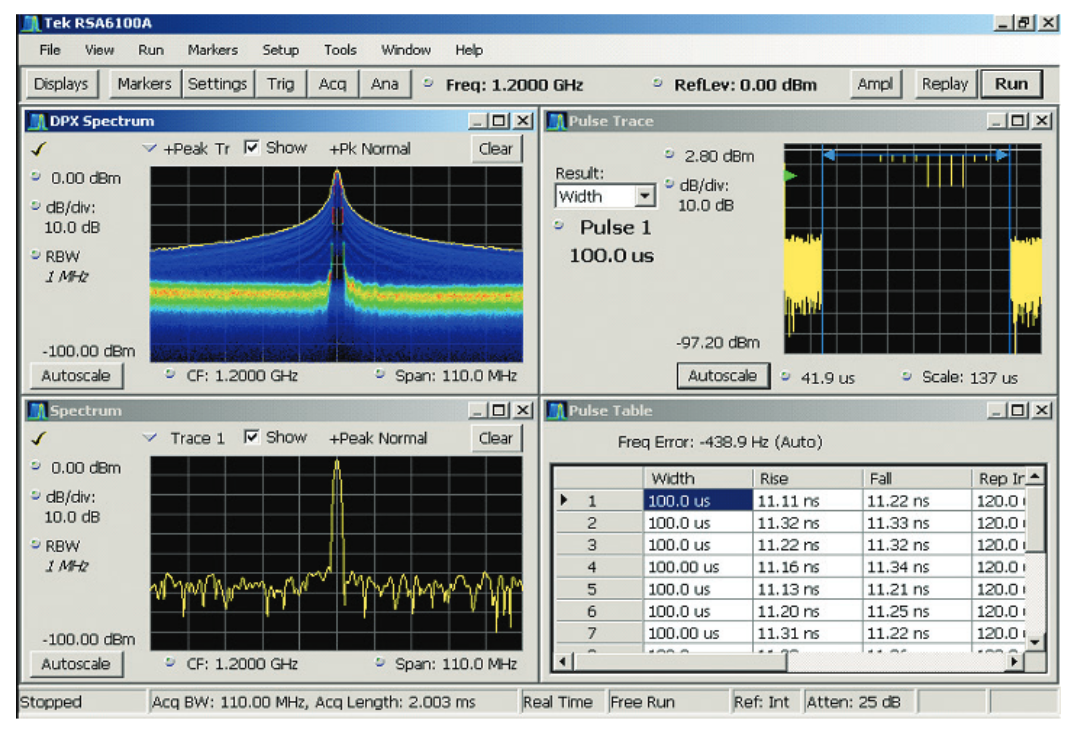
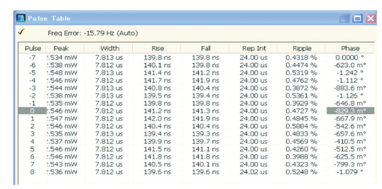
Now the DPX spectrum display is used to “discover” some otherwise invisible artifacts. This Frank Coded pulse has some very interesting characteristics. Each pulse was programmed to have controlled transition times. This should somewhat limit the bandwidth of a CW pulse. The pulse timings can be seen in the pulse table in the lower right of Figure 25 to be 100 µs width and 11 µs rise and fall times. However, the transitions between the different segments of phase are not phasecontinuous. This creates very short-time wide frequency transient spectral components at these transitions.
The entire Sin(x)/x spectrum of the pulse occupies only the very center of the 110 MHz wide standard Spectrum Display in the lower left of Figure 25. This display does not show that there is extended spectral energy present due to the phase discontinuities incorrectly allowed at the transitions between the segments of different phases of the modulation. These phase transitions are only a very small percentage of the pulse duration. A standard spectrum display cannot show the spectral results of these very narrow transitions.
The DPX spectrum display in the upper left dramatically shows the infrequent wideband splatter due to the phase transitions. The dark blue of these excursions denotes that they are very infrequent compared to the central portion of the pulse spectrum.
The spectrum trace is the result of one measurement (depending on the spectrum settings) that may happen once for each pulse, or may integrate for many pulses. The DPX spectrum display with 292,000 individual spectra per second has (for this 100 µs pulse width and 120 µs pulse period) at least six spectrum measurements per pulse with no gaps. This provides discovery of all the spectral energy including the wide splatter from the phase transitions.
DPX spectrum display allows discovery of infrequent or otherwise low probability of intercept signals.
Frequency Mask Trigger (FMT) in the RSA Series
The run-time process engine that is used for DPX spectrum display can be used to monitor the acquisition bandwidth without interruption and trigger the instrument on the incoming frequency spectrum.
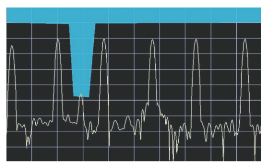
For triggering on specific frequencies at specific amplitudes, Tektronix invented the Frequency Mask Trigger (FMT). The user can draw a mask on the spectrum display. This mask could define a “Trigger if a signal enters here” mask. An example of a mask is in Figure 26. This one is drawn so that in between two of the legitimate signals there is a trigger area drawn. The magnitude of the FFT of a signal is compared again the mask as fast as necessary to satisfy Nyquist criteria. Now if a small signal intrudes on the mask, a trigger is generated which will capture the signal into memory
The signal is being continuously digitized and fed into the acquisition memory. When the data reaches the end of the memory, it seamlessly starts at the beginning of memory and replaces the oldest data. In this circular fashion there is always an entire memory of captured data being updated. When the trigger occurs, the instrument marks the trigger location in memory.
In the same manner as digital oscilloscopes or Logic Analyzers, there are user-specified pre-trigger and post-trigger memory sizes. Once the trigger location is marked in memory,the acquisition will continue until the post-trigger amount of memory is filled.
In this manner the memory can be optimally configured to contain a seamless capture of the events both before and after the trigger.
The mask can be drawn arbitrarily with as many fingers or other shaped areas as desired. Alternatively, the “Autodraw” function can be used to automatically define the spectrum from existing traces in DPX spectrum or Spectrum views with a user-definable frequency and amplitude offset. These points can then be manually modified around specific frequency events of interest.
This mask can trigger on a very small signal at one frequency,while preventing the surrounding huge signals from generating a trigger. A normal power trigger will always trigger on any signal within the IF bandwidth which is above the trigger threshold. The FMT will only trigger on the frequencies specified by the user.
Signals in both Time and Frequency Domains
Some signals may exhibit transient behavior in both the time and frequency domains simultaneously. One example of this is a Phase Locked Loop (PLL) that is marginal in its lock and occasionally unlocks. When it unlocks it may quickly snap back and not unlock again for many hours. Such transient behavior can be very difficult to capture
But complicating the troubleshooting is the likelihood that when unlocked, the oscillator may sweep over a wide frequency range. Such a transient in both time and frequency requires a tool like DPX spectrum display to understand the character of the fault.
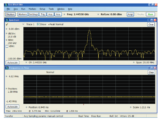
Figure 27 is such an occasionally unlocking PLL. Without DPX spectrum display there is virtually no way to even discover that there is a problem at all. The transient unlock and re-lock takes 150 µs total. This transient repeats about once per second and the duty cycle of the transient is 0.015%. This is why the spectrum trace in the upper window has only the intended carrier and not a clue that there is a problem.
The lower trace is a frequency vs. time demodulation view.If a problem can be located, then its nature can be seen.Next the DPX spectrum display is used to look for any transient problems.
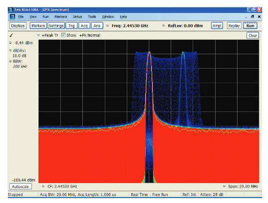
With the DPX spectrum display, the problem is rapidly visible.The very low duty cycle is the reason for such a dim blue color for the transient frequencies while the rest of the spectrum that is continuous shows as very bright red.
Once the problem is discovered to exist, and the frequencies are known where it is doing its work, the FMT can be set up to capture a record only when the transient slips into the right part of the blue display components.
Event Isolation and Analysis
The upper trace in Figure 29 is the same spectrum trace as before, but now it has a FMT set up in the blue box uppermost in the display. That represents where the trigger found the signal, and the spectrum plot displays the frequencies present at that time.
The frequency vs. time display now shows the nature of the transient. The display had been zoomed in to see the detailed shape of the transient. Markers can be used to take exact measurements if needed.
External Threats
There may be many signals external to radar or other electronic systems which will cause problems. When a system utterly ceases to function, it will be known that there is a problem. But some signals may be more subtle such that the radar simply gets the wrong result. This may well be much worse than outright failure.
In the case of the more subtle interference, a method is needed to discover that there is a problem, trigger on it,capture and then analyze it to learn what, and possibly where it is.
Depending on the type of external problem, the techniques for discovering and locating it may differ.
Interference
Interference to a pulsed signal may be hard to find. The next example is the case of a “scanning monitor receiver”located near a radar installation. The Local Oscillator (LO) in the receiver was radiating a harmonic physically near the radar receiver. As the scanner hopped through the band it was monitoring, the harmonic was hopping through the radar pulse frequency
However, initially it was only known that every four seconds or so the radar experienced errors. Figure 30 shows the spectrum as measured by an ordinary spectrum analyzer or VSA. Only the outline of the sine(x)/x pulse spectrum is visible. If the radar could be turned off other signals might be seen, but in this case the interference was only present for limited periods of time, so the radar would need to be turned off for several days.
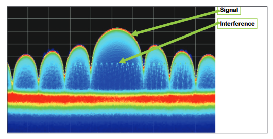
An ordinary analyzer does not have enough spectrum measurements, nor does it combine them so as to be sure not to miss the effects from any one of them.The DPX spectrum display can see all of the spectrum effects. Note how the stepping LO harmonic is easily visible even inside the spectrum lobes of the pulse transmitter. When viewing this on a real RSA Series spectrum analyzer (not a still image as shown here) the Live RF view really makes the interference more visible yet, as the visibility is improved by its movement inside the stationary pulse spectrum.
Unsure which radar test equipment is right for your unique challenge? Our application experts are ready to help you configure the perfect system, combining oscilloscopes and spectrum analyzers for complete signal insight.