Application Note
Engineers designing or validating the Ethernet physical layer on their products need to perform a wide range of tests, quickly, reliably and efficiently. This application note describes various tests that ensure validation, the challenges faced while testing multi-level signals and how oscilloscope-resident test software enables unprecedented efficiency improvements with its wide range of tests, including return loss, faster validation cycles and higher reliability.
It is therefore very important to make the measurements after due signal path compensation on the oscilloscope and probe calibration. Another aspect to consider is the interconnect path between the port and the probe. This should be as short as physically possible.
The Basics
Popularly known as Fast Ethernet, 100BASE-TX has been witnessing rapid growth. With only minimal changes to the legacy cable structure, it offers 10 times faster data rates than the 10BASE-T Ethernet signals. Fast Ethernet, in combination with switched Ethernet, creates the perfect cost-effective solution for avoiding slow networks.
100BASE-TX uses one signal pair for transmission and another pair for collision detection and receive. The transmission occurs at 125 MHz frequency operating at 80% efficiency. It employs a three-level, MLT-3 line encoding signaling scheme as in Figure 1.
Figure 1. 100BASE-TX Multi-Level Transmit 3 (MLT-3) Line Encoding.
Physical layer AOI compliance standards
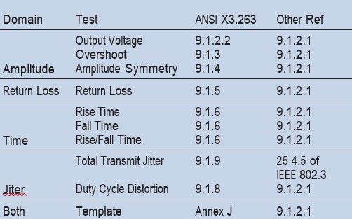
To ensure reliable information transmission over a network, industry standards specify requirements for the network’s physical layer. The ANSI X3.263 and IEEE 802.3 standards define an array of compliance tests for 100BASE-TX physical layer. While it is recommended to perform as many tests as possible, the following core tests are extremely critical for compliance. The core tests are as tabulated below:
Amplitude Domain Tests
These tests are performed on the portion of the random packet signal that generates a pulse going from 0 V to Vout (positive and negative). For reliable measurement, the test is performed on the longest pattern with no transition. The standard describes 112 ns pulse (14-bit pattern) for this purpose. However, these patterns may not be easily available. Results from 12-bit patterns (96 ns pulse) are equally reliable and are used often in testing. Both are positive and negative pulses duration are tested. The signal is depicted in Figure 2.
Figure 2. Amplitude tests performed on long run of logic high levels.
The Annexure J of the ANSI standard defines the peak output voltage as the average positive and the average negative differential output voltage extremes exclusive of any overshoot. For purpose of excluding the extremes from the measurement, the test is performed on the section that is 8 ns away from the transition mid-point. The mean of all waveform points are obtained by averaging the signal with following equation which is mathematically equivalent to a running summation average:
An(i) = An-1(i) + [Xn(i) - An-1(i)]/n
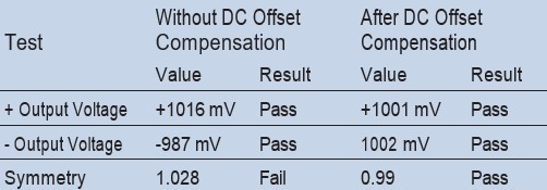
Amplitude values are calculated for both positive and negative pulses and are compared against the standard value. The Vout values should lie between 950 mV and 1050 mV as specified in the standard. The standard defines waveform overshoot as the percentage excursion of the differential signal transition beyond Vout. The limit specified for the overshoot value is < 5%. The ratio of +Vout and -Vout values is calculated to provide the signal amplitude symmetry. As defined by the standard, this value should lie between 0.98 and 1.02.
With margins < ±5%, it is important that the measurement is accurate and the acquisition errors are minimized. While performing these measurements, attention should be paid to interconnects and the oscilloscope measurement system. With voltage levels of 2 Vpk-pk, even 1% gain accuracy in the oscilloscope implies errors up to 20 mV. Figure 3 demonstrates the advantage of performing the test with full dynamic range for each level of transmission.
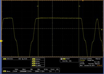
Figure 3. Optimized setup for dynamic range with increased resolution on the high level.
In this case, testing with full dynamic range eliminated 5 mV of error (1.023 V versus 1.018 V). This can make a difference when the margin is only 100 mV.
If the DC Offset introduced by the differential probe is not properly compensated, this error can quickly add up to large numbers when compared with the ±50 mV margin defined by the standards. The measurement errors caused by the DC Offset can be best described by the following example:
DC Offset = 15 mV; +Vout = 1001 mV; -Vout = -1002 mV
Tektronix differential probes (TDP) have an AutoZero feature which automatically eliminates DC offset errors in the probe signal path.
It is therefore very important to make the measurements after due signal path compensation on the oscilloscope and probe calibration. Another aspect to consider is the interconnect path between the port and the probe. This should be as short as physically possible.
Return Loss Test
The return loss test provides an indication of the performance of the transmission system. The standard defines the minimum amount of attenuation the reflected signal should have relative to the incident signal.
In order to ensure interoperability, the standard also specifies the impedance of the cabling system under which the return loss is tested. The environment is specified as 100 W ± 15%. As a result, the test needs to be performed over the impedance range of 85 W, 100 W and 115 W.
The test is performed for transmit as well as receive pairs. The device is set to transmit scrambled signals in Idle or Halt Line state.
The screen shot, Figure 4, shows the three plots (85/100/115 W) for 100BASE-TX transmit pair.
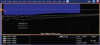
Figure 4. 85/100/115 W plots for the Return Loss measurement.
Time Domain Tests
The reference waveform for this test needs to be carefully chosen such that the rise and fall times of the signal are minimally affected by the inter-symbol interference. It is therefore imperative to choose the longest pulse that is preceded and succeeded by at least two consecutive symbols at baseline voltage.
For this reason, the tests are performed on the portion of the random packet signal that generates a pulse going from 0 V to Vout, with at least 10 bit times of no transition preceded and succeeded by at least 2 symbols at baseline voltage. Both positive and negative pulses of 80 ns (10 bits times 8 ns)duration are considered.
The signal is depicted in Figure 5.
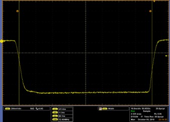
Figure 5. 10 consecutive bits for rise/fall time measurements.
Signal is termed “rising” when transitioning from the baseline voltage to either +Vout or -Vout. Likewise, signal is “falling” when transitioning from either +Vout or -Vout to the baseline voltage. The rise and fall times are measured between 10% and 90% of the transition from baseline to Vout.
The rise and fall times should be between 3 ns and 5 ns. The standard also says that the difference between the maximum and minimum of all measured rise and fall times shall be less than 500 ps.
Two factors are extremely critical in robust rise and fall time measurements. The bandwidth of the oscilloscope and probe should be adequate to measure the rise times with minimal error. The following table describes the reduction in error as bandwidth of the oscilloscope increases.
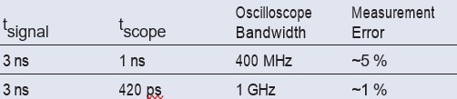
The second factor of importance is the sampling rate. This becomes very significant while validating the difference between the rise time and the fall time. With pass/fail determination at 500 ps, the sampling rate should be at least 5 GS/s to ensure reliable results.
Jitter Test
The transmit jitter includes contributions from duty cycle distortion and the baseline wander. Peak-to-peak jitter is measured using scrambled IDLEs or HALT line state.The most common method for the jitter test is measuring the width of the accumulated set of points, often done with infinite persistent modes accumulating points until a certain number of “hits” are measured. A distribution histogram is made and the peak-to-peak can be inferred from minimum and maximum values in the tails of the histogram.
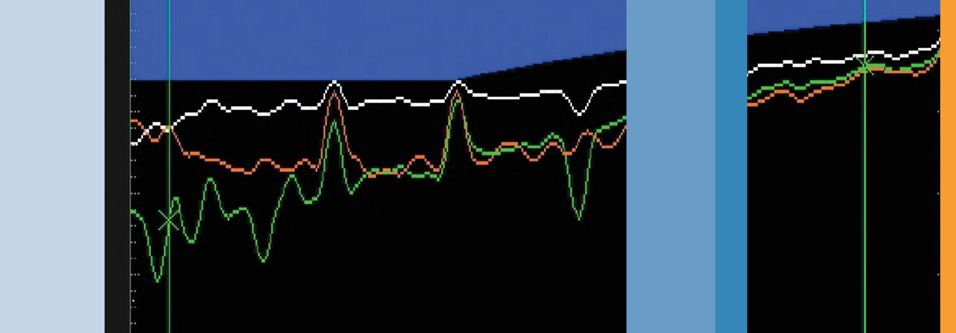
Being a three-level signal, it is extremely important to quantify the peak-to-peak jitter at both, the upper and lower, crossovers and determine the worst-case value of the two. Determining peak-to-peak jitter based on only one crossover can lead to inconclusive and, at times, incorrect results as shown in Figure 6.
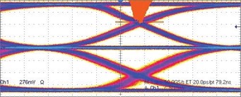
Figure 6. Peak-to-peak jitter with single voltage crossing.
Duty Cycle Distortion Tests
In order to quantify the duty cycle distortion (DCD), the system should be driven with a determined clock-like pattern (such as 0-1-0-1-0-1-0-1). While selecting the pattern, it is also important that there is minimal inter-symbol interference that could affect measurements.
For these reasons, DCD is measured at portions of the signal where the four successive MLT-3 transitions generated by a 0-1-0-1-0-1-0-1 NRZ bit sequence that is preceded and succeeded by at least two consecutive symbols at the baseline voltage.The signal is depicted in Figure 7.
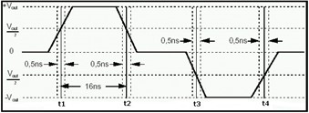
Figure 7. Test pattern for Duty Cycle Distortion test.
The pattern has widths of positive and negative polarity MLT-3 pulses that are nominally 16 ns wide. The standard specification states that the deviations of the 50% crossing times from a best-fit grid of 16 ns spacing shall not exceed ±0.25 ns.
This requirement is easily verified in terms of a peak-to- peak specification. Given the 50% crossing times tn (refer to Figure 25.1.3-1 in the Ethernet specifications), compute the maximum of the Tx.
T1 = t2 - t1 - 16 ns
T2 = t3 - t2 - 16 ns
T3 = t4 - t3 - 16 ns
T4 = t3 - t1 - 32 ns
T5 = t4 - t2 - 32 ns
T6 = t4 - t1 - 48 ns
The maximum of Tx is the peak-to-peak DCD and should not exceed 0.5 ns to pass the test.
The scrambled random test pattern usually includes the 0-1- 0-1-0-1-0-1 pattern. A traffic generator may be used if absent in the random packet. In such case, the scrambler needs to be turned off and the required pattern is sent across.
AOI Template test
A mask test is often used to quickly verify that the transmitted signal meets industry standard requirements and is performed on scrambled HALT Line state.
For 100BASE-TX, the AOI Template Mask is defined so that the signal distortions such as overshoot, jitter, incorrect rise and fall times, etc., will cause the mask test to fail. The specifications in Annexure J also specify a tolerance of 5% on the mask geometries.
It is important to recognize that dynamic range issues discussed earlier in the document also affect this test. Another aspect to reckon is that the display resolution gets doubled when the signals and masks are amplified over the vertical scale. It is therefore more reliable to perform the mask test separately – positive and negative, as shown in Figure 8 and 9.
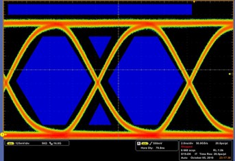
Figure 8. Testing positive side for AOI Template test.
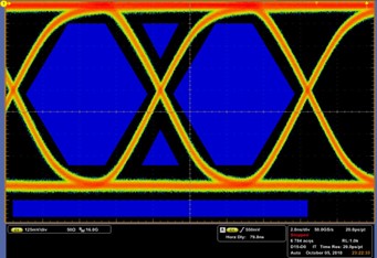
Figure 9. Testing negative side for AOI Template test.
Preparing for the tests
In order to perform the complete suite of tests described previously, you would require a digital storage oscilloscope, differential probes and a test fixture. A software tool may be needed to configure the port under test to transmit random test packets.
a. Digital Oscilloscope: While choosing the right oscilloscope, it is important to consider the rise time, sampling rate and acquisition technique of the oscilloscope. As discussed, it is important that the rise time of the measurement system (right up to the probe tip) is of the order of 400 ps. This would ensure minimal error in measurements ensuring accurate and reliable test results.
Also, the test limits of duty cycle distortion test and the rise/fall symmetry tests demand high-sample rate. It is imperative to have a sampling rate in excess of 5 GS/s in order to offer the resolution required for these measurements.
A good fit for such applications is an oscilloscope in the DPO7000 Series that offers at least 1 GHz bandwidth with 420 ps rise time (at the probe tip) and 10 GS/s sampling speed.
b. Differential Probe: The 100BASE-TX is a differential transmission system. Using a pair of single-ended probes to make the measurement requires accurate de-skewing and careful matching of the pairs. Failure to do so can lead to undesirable artifacts in the measurement resulting in erroneous test results.
Tektronix offers a full suite of differential probes to choose from which include the TDP1500, offering 1 GHz system bandwidth, to the TDP3500 that offers 3.5 GHz bandwidth to serve 100BASE-TX test needs. In order to perform Return Loss tests, two differential probes are required.
c. Arbitrary Waveform Generator: The Arbitrary Waveform Generator, or AWG, is used for the Return Loss test and is also used in the Common-mode Rejection test. The AWG is also used for several tests for other Ethernet standards such as 1000BASE-T. An AWG with a sample rate of 250 MS/s or above is ideally suited for Return Loss tests.
d. Test Fixture: The standard describes the fixturing requirements for performing the tests. It is important to recognize that the integrity of the fixture directly affects the reliability of the tests. The Tektronix TF-GBE-BTP 1000/100/10BASE-T Basic Ethernet Test Package is well suited for testing the physical layer. Carefully laid interconnects help minimize unwanted exposure to cross- talk and other side-effects. It is extremely important that the distance between the port under test and the probe- interconnect-point are not more that an inch.
To summarize, choose a digital storage oscilloscope with at least 400 ps rise time (> 1 GHz BW), sampling rates in excess of 5 GS/s. Ensure you are using a differential probe that offers at least 400 ps rise time while in use with the oscilloscope. An AWG with sample rate of 250 MS/s or above can be used for many tests. Use a well-designed test fixture that minimizes distance between probing points and the DUT.
Getting the Scrambled Random Test Pattern
There are two predominant methods of generating the scrambled random test pattern from the port under test:
1) Configuring the port registers:
The port registers provide a convenient method to set the port to transmit the scrambled pattern. The registers can be accessed using special software available from the silicon- provider. Contact your silicon-provider for more information on accessing port registers.
Once the port is configured to generate the random sequence, connect as described in Figure 10.
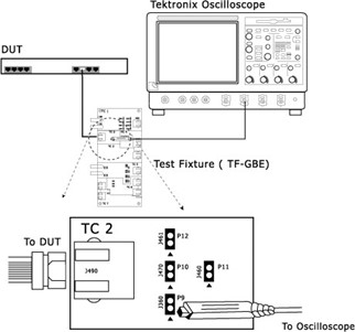
Figure 10. Test setup without link partner.
2) Using a Link partner:
100BASE-TX implementations send scrambled idle random sequence upon detecting a link. Connecting the port-under- test to another 100BASE-TX device (called link partner) would initiate the sequence generation.
A link partner could be a computer, a hub or a more sophisticated traffic generator. The oscilloscope’s Ethernet port could also be used as a Link partner by setting it to 100 Mb/s and turning the auto-negotiation OFF.
The scheme of connections can be described as in Figure 11.
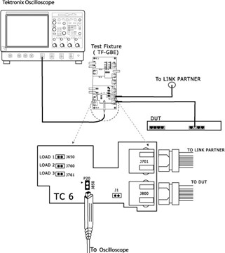
Figure 11. Test setup with link partner.
3) Test Setup for Return Loss Test
For this test, the port is configured to generate the scrambled sequences. The test setup is described in Figure 12.
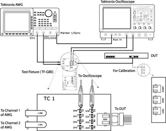
Figure 12. Test setup for Return Loss measurement.
Performing the tests
The usual test process essentially involves four discrete steps as follows:
- Recalling oscilloscope setups
- Performing the test and its related measurements
- Exporting screen-shots
- Documenting results
The challenge is the MLT-3 signals need to be characterized for both, the positive-going as well as the negative-going pulses.
- The number of tests that need to be performed for each signal behavior almost doubles as a result of the need to perform the tests on both sides. Thus, different setups are required for positive-going pulses and negative-going pulses.
- The measurements need to be performed on properly defined gated regions. Human interventions can lead to non-repeatability and, at times, subjective measurements.
- Tests, such as the jitter tests, require fine-tuning of the settings in order to perform accurate measurements. The test needs to measure jitter on upper cross-over as well as the lower cross-over and the worst case needs to be considered for test purposes. Again, subjectivity introduced by human-intervention can lead to inconsistent results.
Compliance Test Software
Engineers designing or validating their 10/100/1000BASE-T physical layer need to perform thorough validation in-house validation. TDSET3 Ethernet Compliance Test Software enables performing a wide range of tests reliably and efficiently.
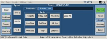
Figure 13. 100BASE-TX measurement selection.
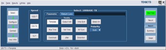
Figure 14. 100BASE-TX measurement configuration,
Performing the tests using TDSET3
Users can select the entire range of tests by clicking on “Select All” button and run the tests at a press of a button. The return loss tests are invoked when the Return Loss tab is pressed.TDSET3 enables testing, per the standard, including scaling of mask to 0.95 and 1.05. The user interface allows flexibility in setting up the tests and eliminates confusion.
Pressing the Run Test button starts the test process and after performing all the tests, presents the results as shown in Figure 15. Pressing Result Details button provides more information on limits and measured values.
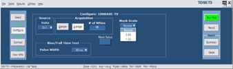
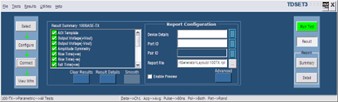
Figure 15. TDSET3 Results panel with pass/fail status.
Report generation is instantaneous at the press of a button. The reports can then be easily converted into popular formats such as portable document files and others. Reports can also be documented in comma-separated- variable format by pressing the Summary button. This is very useful when testing multiple ports and documenting them as a summary. The .csv format allows easy documentation in popular tools like Excel and many others.
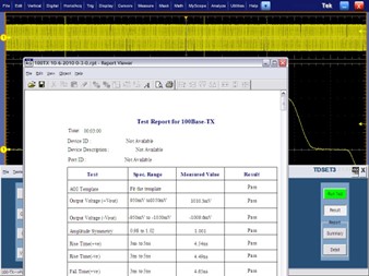
Figure 16. Test Report for 100BASE-TX.
Benefits:
The TDSET3 Ethernet Compliance Test Software cuts validation cycles from hours to minutes. The innovative oscilloscope-based return loss test enables efficient use of resources. With plots for 85/100/115 W impedances, pass/ fail testing and integration with the automatic report generator, Return loss tests can be performed quickly and reliably.
Summary
Engineers designing or validating the Ethernet physical layer on their products need to perform a wide range of tests, quickly, reliably and efficiently. The large numbers of tests, coupled with multi-level signals impose several challenges to the test engineer. Tight margins require careful measurements and thorough understanding of error contributors.
TDSET3 enables efficiency improvements by performing a wide range of tests quickly and reliably. The innovative oscilloscope-based Return Loss helps use resources efficiently and performs tests for 85/100/115 W impedances.