Abstract - Impulse Response can be performed on a complete radar transmitter as a measure of transmitted pulse quality.Several types of pulse distortions that are difficult to discover by traditional quality measurements can be readily quantified.Errors such as the amplitude of a secondary reflected response relative to the main pulse, or incidental periodic modulations can be accurately measured.
I. INTRODUCTION
Traditional measurement of the quality of a linear FM chirp has used Frequency Linearity or Phase Linearity. The linearity of frequency or phase of the chirp tells only part of the story. If a reflection or other time-related mechanism results in a delayed copy of the intended pulse (a secondary pulse) added to the main pulse, the linearity measurements may not easily discover the problem. Also, if a chirp pulse has periodic incidental modulation (particularly amplitude modulation), such an error may also very difficult to determine.
Impulse Response has commonly been included in the measurements made by vector network analyzers. As such, it is performed on components or assemblies as a forward transfer measurement. The Network Analyzer supplies the swept RF stimulus in addition to measuring the resultant output signal.
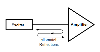
A measurement of the quality of a complete radar transmitter can be made using the FM chirp from the radar's own exciter as the swept RF source. In this manner, the quality of the generated chirp as well as all modules that the chirp passes through will be tested together as a complete assembled radar. This Impulse Response measurement is also called Time Sidelobe measurement.
The most obvious measurement is of a reflected and delayed copy of a chirp included with the main pulse. Such a secondary pulse can be simultaneously measured for both time delay and relative amplitude by plotting the impulse response of the main chirp pulse. This is functionally equivalent to a TDR using the chirp itself as the excitation signal.
Another defect, which this process can easily discover and measure, is incidental periodic modulation. Incidental modulation adds sidebands to the sweeping RF carrier. These sidebands effectively create lower amplitude copies of the chirp that appear as pulses both preceding and delayed behind the main chirp.
All of these defects would appear as false responses in a radar receiver.
II. THE IMPULSE RESPONSE MEASUREMENT
A. The Time-Window.
After the incoming signal is digitized, a time window is applied to the samples to reduce undesired sidelobes that would be generated by the Discrete Fourier Transform for a signal that is not continuous. For this purpose a Taylor window provides a good compromise of main lobe width and reduced sidelobe generation. Equation (1) describes a Taylor window function [2].
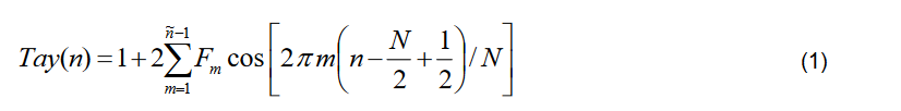
For values of n = 0 to N-1
B. The Basic Impulse Response (IPR).
The windowed set of time samples is then transformed into a frequency-domain spectrum. This can be accomplished by any of several Discrete Time Transform processes, including the Fast Fourier Transform (FFT).
This spectrum data is then multiplied by the complex conjugate of a representation of an ideal chirp as was expected to have been transmitted.
In a practical implementation of a measurement tool, this ideal chirp can be mathematically estimated using the actual incoming signal, or it can be entered by the equipment operator for increased measurement accuracy.
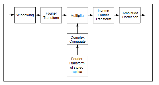
The multiplication de-chirps the acquired pulse. After de-chirping, the Inverse Frequency Transform is performed to transform the result back into the time domain. This is now the traditional Impulse Response of the incoming chirp signal which passed through the radar system [1].
C. The Resulting Amplitude Reduction of the Secondary
Since the Impulse Response measurement is calculated only over the duration of the main chirp pulse, the reflection pulse will be truncated by an amount equal to the delay time of the reflection from the main pulse.Additionally the time window function adds more loss as the time delay becomes larger.
This reduction in the processed amplitude of the secondary pulse will cause an error in the reported measurement result for its amplitude if no correction is applied.
D. Amplitude Correction1
First the attenuation factor α(td) is calculated as the energy of the secondary pulse divided by the energy of the main pulse using (2). This is how much smaller the secondary pulse is than it would have been if it were not reduced by the signal processing.

Where Em is the energy of the main pulse Eg is the energy of the secondary pulse, and td is the delay time that reduces the energy measurement for the secondary pulse. The correction curve is calculated individually for each measurement and applied in the far right block in Figure 1.
As the measurement limit of 50% of the pulse duration is approached, the correction factor can approach 3 dB for the Taylor window [2] chosen here.
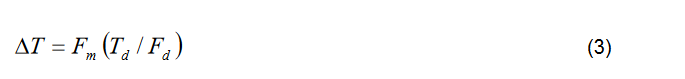
E IPR Results for a Reflection Measurement
In Figure 3 the amplitude correction has been applied and the measurement result shows the secondary pulse (time sidelobe) as 42.40 dB below the main pulse (main lobe).
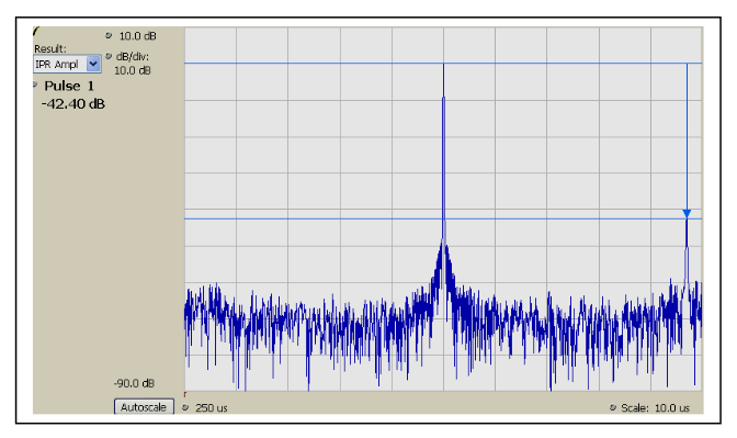
A reflected pulse will be displayed as one time sidelobe separated by twice the path delay from the main lobe.
1 Reference [5] describes the complete amplitude correction theory and method for impulse response. Only the correction equation itself is shown here.
F. IPR Measurements for Other Pulse Defects.
Measurements which include a secondary reflected pulse are one use of this measure of quality. There are other pulse conditions that also can be measured using this method. One example is a chirp pulse that has incidental sinusoidal modulation.
The relationship between the impulse sidelobe delay time and the frequency components of the chirp is given in (3)
Where ∆T is the time difference between the time sidelobes and the main lobe, Fm is the frequency of the incidental modulation, Td is the duration time of the chirp, and Fd is the frequency sweep width during the chirp.
G. IPR Measurement Time Resolution
The time resolution in the measurement is determined by the width of the main lobe of the impulse response.
The lobe width is primarily the inverse of the frequency width of the chirp. Additionally the required time window function will increase the lobe width [1].
H. Comparison with Traditional Measures of Chirp Quality
Such a pulse exhibits modulation sidebands on both sides of the carrier in the frequency domain. For a chirp pulse, this effectively has a secondary pulse both preceding and following the main pulse in the time domain.
The example displayed in Figure 4 has a chirp width of 100 MHz, time duration of 10 microseconds, and incidental AM modulation at 15 MHz rate. This results in time sidelobes at 1.5 microseconds on both sides of the main lobe.
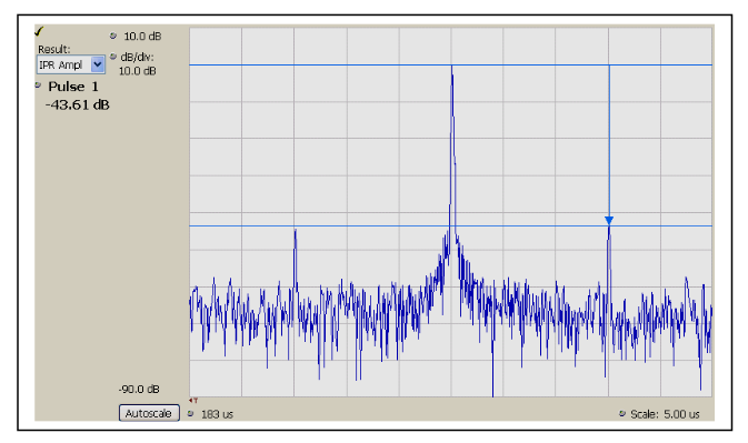
A plot of frequency versus time for a chirp will reveal only gross errors. The plot in Figure 5 shows no indication of the amplitude modulation sidebands present at all frequencies. It also cannot show any amplitude variations themselves.
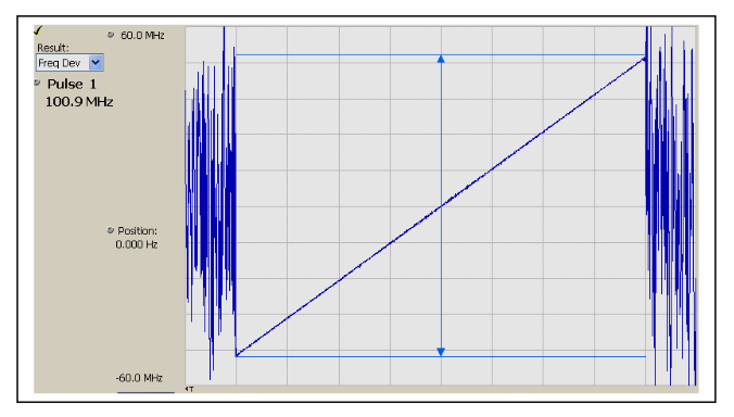
Figure 6 is a more sensitive measure of frequency errors, but there is still no indication of the modulation sidebands. This measurement is produced by subtracting an ideal chirp waveform from the measured pulse, leaving only the errors from a perfectly linear chirp. This plot has been expanded revealing only the noise included in the measurement bandwidth.
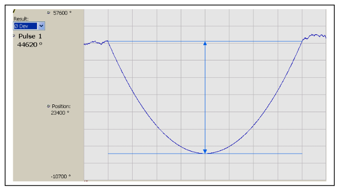
Phase is always a more sensitive measure than frequency. In Figure 7 the phase shows no indication of the amplitude modulation. The sidebands due to the modulation are not visible.
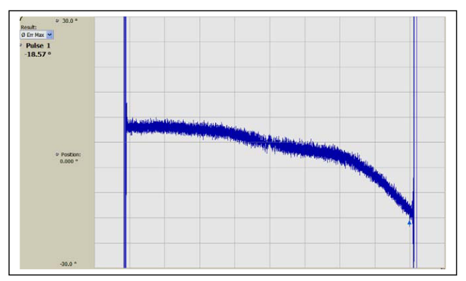
Phase error, shown in Figure 8 is produced by subtracting the ideal phase parabola from the measured phase. Even in this most sensitive measurement, there is a long-term phase error seen, but no effect from the amplitude modulation.
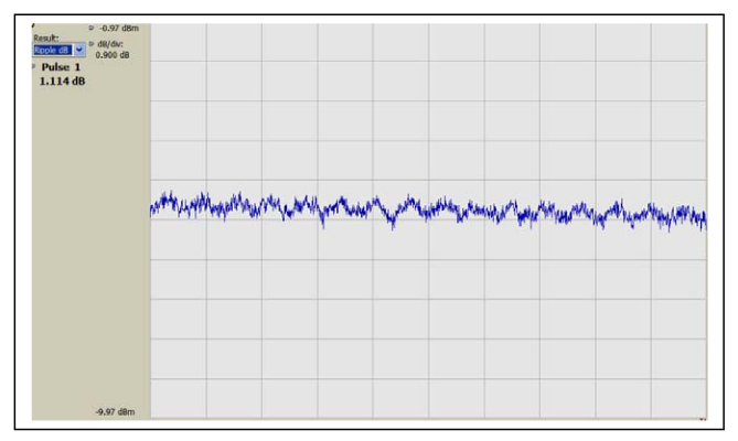
Only a plot of pulse amplitude versus time in Figure 9 shows any indication of this low-level AM. Since the modulation is only a few dB above the broadband noise, it is difficult to measure the character of the modulation. It is unclear if this is a single-frequency sinusoid, or is largely noise.
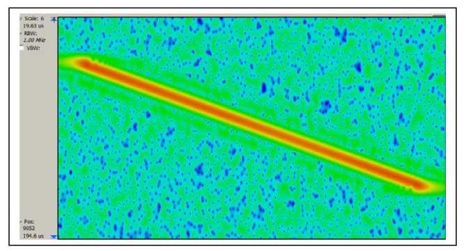
Using a Spectrogram (a set of FFT spectra over time placed one above the other to show time vertically, frequency horizontally, and amplitude as color or intensity) is limited by the FFT process. For the 110 MHz bandwidth used for these measurements, the available time resolution is one FFT frame. This is approximately 13 microseconds. This can not resolve the 1.5 microsecond delay time. The available frequency resolution is also insufficient. This limit comes from using the FFT without the time compression resulting from the impulse response mathematics.
These traditional measurements of chirp quality can be compared to Figure 4 to demonstrate the superiority of the impulse response measurement as a measure of the quality of the linear FM radar chirp.
III. CONCLUSION
Impulse Response is an improved method of measuring the quality of FM chirp radar pulses. This can be implemented as a signal analyzer measurement utilizing the radar chirp itself as the swept frequency excitation signal.
ACKNOWLEDGMENT
The authors wish to acknowledge the assistance provided by Michael Nelson, Darren McCarthy, John Turpin and Marcus DaSilva in the preparation of this paper.
REFERENCES
[1] Charles E. Cook & Marvin Bernfeld, "Radar Signals – An Introduction to Theory and Application", 1993, Artech House.
[2] Walter G. Carrara et. al., "Spotlight Synthetic Aperture Radar", 1995, Artech House.
[3] Alan Oppenheim & Ronald Schafer, "Discrete-Time Signal Processing", 1989, Prentice-Hall.
[4] T. C. Hill, "Measuring Modern Frequency Chirp Radars", Microwave Journal Magazine, Vol 51, No. 8, August 2008.
[5] T. C. Hill & Shigetsune Torin, "Amplitude Correction for Impulse Response Measurement of Radar Pulses", Tektronix White Paper 37W-25527-0.