As you may have noticed if you’re regular reader of Evaluation Engineering or other electronics engineering news outlets, we recently released a firmware upgrade for the 5 and 6 Series MSOs that unlocks a new analysis tool called Spectrum View. You can read more about how it gives you a frequency domain display for each of your analog channels with independent time- and frequency domain controls here.
If you are an experience scope user, you most likely have at one time or another used the FFT (fast fourier transform) feature on your scope with varying degrees of success. For this post, we look at how traditional scope FFTs compare to Spectrum View. Then in Part 2 we take look under the covers at how Spectrum View actually works and in the process opens up a whole new world of spectrum analysis capability for scope users.
Although spectrum analyzers are designed specifically for viewing signals in the frequency domain, they are not always readily available. Scopes, on the other hand, are almost always nearby in the lab so engineers tend to rely on scopes as much as possible. This is one of the key reasons why oscilloscopes have included math-based FFTs (fast fourier transforms) for decades.
Unfortunately, FFTs are notoriously difficult to use for two reasons:
First, for frequency domain analysis spectrum analyzer controls like center frequency, span and resolution bandwidth (RBW) make it easy to define the spectrum of interest. In most cases, however, oscilloscope FFTs only support traditional controls such as sample rate, record length and time/div, making it difficult get to the right view.
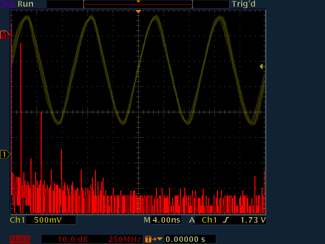
Second, FFTs are driven by the same acquisition system as that used for the analog time domain view. This means that speeding up the time scale in the time domain reduces resolution in the frequency domain. As a result, with conventional FFTs it’s virtually impossible to get optimized views in both domains. For example, in the screen shot below from a TDS3000, the time domain waveform is seen clearly, but FFT resolution is inadequate to see meaningful details.

Frequency modulation details are more visible in the image below with a slower time scale setting, but the time domain trace is now practically unusable.

By way of comparison, Spectrum View provides the ability to adjust the frequency domain using familiar center frequency, span and RBW controls. And because these controls do not interact with the time domain scaling, it is possible to optimize both views independently as shown below.

On-screen indicators (spectrum time) show the source of the spectrum on the waveforms. The ability to synchronize the two domains is useful for correlating signal activity on a board with EMI emissions, for example.
Conventional FFT Tradeoffs
The challenges with conventional FFTs go beyond ease of use. To illustrate the performance tradeoffs engineers must consider, let’s say we have a tone at 900 MHz and want to view its phase noise out to 50 kHz on either side of the tone with 100 Hz resolution. Ideally, the spectral view should have the following settings:
- Center frequency: 900 MHz
- Span: 100 kHz
- RBW: 100 Hz
With a traditional scope FFT, horizontal scale, sample rate and record length settings determine how the FFT works and must be considered holistically to produce the desired view. Horizontal scale determines the total amount of time acquired. In the frequency domain, this determines your resolution. The more time you acquire, the better resolution you get in the frequency domain.
To resolve 100 Hz, we need to acquire at least (1/100 Hz) = 10 ms of time. However, in reality we need to acquire nearly double that amount of time. In theory, FFTs are supposed to be applied to infinitely long signals. Since this isn’t possible, the beginning and end of the acquisitions introduce discontinuities (and thus error) into the resulting spectrum. To minimize discontinuities, the acquired record needs to fit in an FFT “window.” Most FFT windows have a bell or Gaussian shape where the ends are very low and the middle is high, meaning the spectrum must be primarily driven by the middle portion of the acquired data. Each window type has a constant associated with it. For this example, using a Blackman-Harris window type with a factor of 1.90 would require that we acquire 19 ms (10 ms*1.9 = 19 ms) of time.
Sample rate determines the maximum frequency in the spectrum, where Fmax = SR/2. For a 900 MHz signal, we need a sample rate of at least 1.8 GS/s. Using the analog sampling on the 5 Series as an example, we would sample at 3.125 GS/s (first available sample rate above 1.8 GS/s).
Now we can determine the record length. This is simply Time Acquired * Sample Rate. In this case, it’s 19 ms * 3.125 GS/s = 59.375 Mpoints record length.
Depending on the instrument, this record length may not even be available. Even if the scope has sufficient record length, many scopes limit the maximum length of an FFT because it is computationally intensive. For example, many previous-generation oscilloscopes have a maximum FFT length of approximately 2 Mpoints. Assuming you still want to see the 900 MHz signal (which requires the high sample rate), you’d have to acquire approximately 1/30th of the desired time resulting in 30 times worse resolution in the frequency domain.
As this example illustrates, setting up a desired view requires an appreciation of the complex interactions between horizontal scale, sample rate, and record length. Moreover, the reality of finite record length forces undesirable compromise and observing high-frequency signals with good resolution in the frequency domain requires extremely long data records which are often unavailable, or expensive and time-consuming to process. Although some spectral analysis packages attempt to manage these tradeoffs, all oscilloscope FFT implementations to date face the limitations described above.
Stay tuned for Part 2 of this blog series to learn how Spectrum View provides spectrum analysis without the inherent tradeoffs of FFTs.