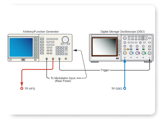
The test, alignment, and troubleshooting of a conventional AM/FM radio is a fundamental skill for any electronic technician. These tasks, whether performed as a classroom exercise or in a commercial repair shop, require a good working grasp of DC and AC electronic basics and RF behavior. Equally important, the procedures call for a thorough knowledge of the core measurement tools that serve radio work and many other applications throughout the industry: the signal generator and the oscilloscope1. A typical measurement setup using these tools is shown in Figure 1.
In this application note we will see how these two tools support radio measurements ranging in frequency from the audio band to the FM spectrum (88-108 MHz). The signal generator in our examples will be an arbitrary/function generator, a general-purpose instrument with the bandwidth that radio work demands. The oscilloscope will be a digital storage oscilloscope with comprehensive triggering features and of course, bandwidth sufficient to accurately capture signals in the RF and IF sections of the radio.
1 A DC voltage/current meter is also used but will not be required for the measurements covered here.
The Arbitrary/Function Generator
The application examples in this document will use an arbitrary/function generator (AFG) as their input signal source. The AFG uses a powerful architecture that relies on direct digital synthesis to produce virtually any waveform shape, as well as noise signals and more. Most traditional function generators use analog oscillators to produce a few fixed waveform types: sine, square, sawtooth, and so on. In contrast, the AFG stores and reads out waveform sample points to reproduce low-distortion signals at a wide range of frequencies.
The specific instrument used in this application note is a Tektronix AFG3252. It has two independent outputs and a sine wave frequency range up to 240 MHz. The AFG3252 incorporates all the usual preset function generator waveforms and many more. In addition its memory accepts user-defined waveforms of any arbitrary shape. The instrument also offers built-in frequency sweep and other features that simplify radio test and troubleshooting tasks.
1 A DC voltage/current meter is also used but will not be required for the measurements covered here.
The Oscilloscope
The oscilloscope will be a Tektronix TDS2024B, a digital storage oscilloscope (DSO) whose 200 MHz bandwidth is more than adequate for AM/FM radio applications. Although the TDS2024B has four input channels, a two-channel instrument is equally capable of doing the job. The TDS2024B’s independent trigger input, too, will be useful in some of the application examples that follow. The oscilloscope is equipped with lowcapacitance (17 pF) passive P2220 probes designed for the TDS2000B Series.
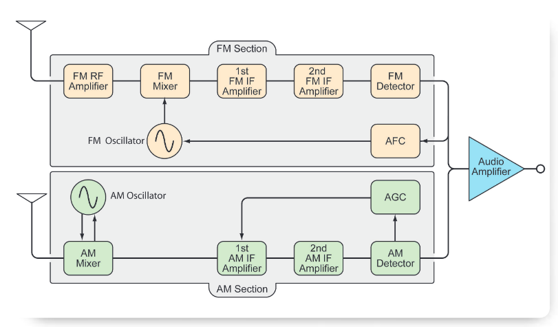
The Radio Circuit Under Test
Figure 2 depicts the block diagram of the superheterodyne radio that is the subject of this application note. The radio is a Model AM/FM-108K receiver available in kit form from Elenco™ Electronics. The circuit and measurement principles in the examples that follow are applicable to almost any transistorized AM/FM radio receiver. For the sake of simplicity, this block diagram and the subsequent discussions assume a monaural radio, switchable to either the AM or FM band, with just one audio output for either type of broadcast.
The superheterodyne radio operates by converting incoming signal frequencies to a lower frequency through a process known as heterodyning. The receiver mixes a signal from a built-in local oscillator with the incoming signals from the antenna. The two different frequencies are multiplied to produce two new signals, one at the frequency sum and the other at the frequency difference of the two original signals.
The resulting difference signal, now called the IF, continues through the radio circuit where it is filtered, amplified and demodulated to produce the final audio output. The intermediate frequency of the AM section of our example radio (and most other consumer AM radios) is 455 kHz. The intermediate frequency for most FM receivers is 10.7 MHz.
The application examples that follow will examine some key test steps for the super-heterodyne receiver. Each step is a common radio measurement that uses the AFG and the oscilloscope to full advantage.
Note: all of the suggested AFG amplitude values were determined empirically using the specific radio brand and model mentioned above. It will almost certainly be necessary to experiment with these values when testing other types of radio devices. The key is to optimize the AFG settings for the real needs of the device under test.
AM Section Intermediate Frequency (IF) Bandwidth Measurement
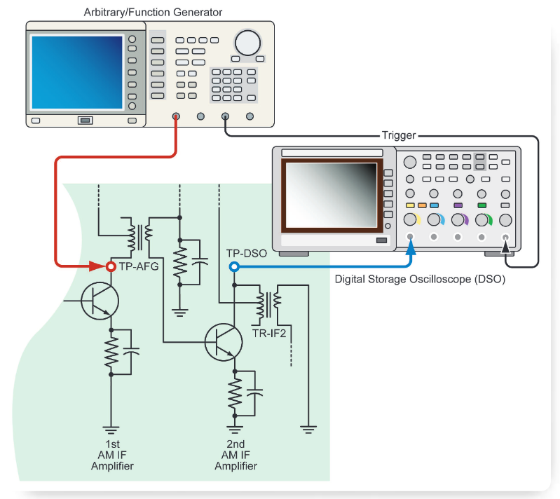
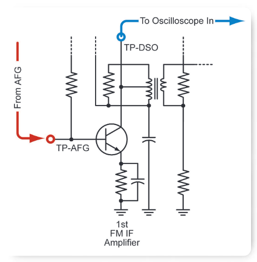
The purpose of this test is to confirm that the IF amplifier circuit can deliver the 455 kHz IF signal without significant attenuation. The test also determines the "3 dB" points; that is, the frequencies on either side of 455 kHz at which the signal’s amplitude is reduced by 3 dB.The measurement setup is shown in Figure 3. The schematic is simplified; it deliberately omits components and connections not involved in this test. The AFG feeds the IF signal to the circuit at TP-AFG, the output of the 1st IF amplifier transistor. The oscilloscope extracts the resulting signal from TP-DSO, the output of the 2nd IF amplifier. By sweeping the AFG frequency between two "boundary" frequencies, we can determine the effective frequency response of this latter amplifier.
It is common practice to couple the signal source output to the radio test points through a .001 µF capacitor. This prevents the flow of DC current in either direction—from the signal source into the radio circuit or from the radio back into the source. However, this is an optional step.
| Start frequency | 430 kHz |
| Stop frequency | 480 kHz |
| Amplitude | Empirically determined in previous step |
| Sweep | 2.5 seconds |
| Return | 2.5 seconds |
| Press "More" | (Displays next set of parameters) |
| Hold | 0 (zero) seconds |
| Type | Linear |
| Press "More" | (Displays final set of parameters) |
| Mode | Repeat |
| Source | Internal |
| Slope | Pos |
Table 1.
In addition to the signal path I/O connections, connect the Output TTL signal on the front panel of the AFG directly to the oscilloscope’s External Trigger input. This keeps the oscilloscope’s acquisition synchronized to the AFG signal, even as the signal frequencies change during the test.
The oscilloscope is of course connected to TP-DSO through a probe such as the Tektronix P2220. The probe’s input capacitance should be small to avoid "detuning" TR-IF2, the output transformer of the 2nd AM IF Amplifier. The P2220 has an input capacitance of 17 pF.
Establish a Baseline Waveform
Select a Sine waveform on the AFG, set the mode to "Continuous" and set the output frequency to 455 kHz. With the radio circuit power on, adjust the AFG output amplitude until the waveform on the oscilloscope reaches the recommended value for the specific radio under test. In our example radio the empirically determined value—the output of the 2nd IF amplifier— is 4 volts p-p. It may be necessary to simultaneously adjust TR-IF2 to maintain maximum output while increasing the AFG amplitude. The resulting waveform is the baseline response of the 2nd IF Amplifier at 455 kHz.
Set Up a Frequency Sweep
The whole point of this measurement is to drive the IF circuit with a range of frequencies and capture its varying amplitude response. The AFG’s sweep capability makes this easy. It can be programmed to change its output frequency smoothly and continuously between two end points.
Set the run mode on the AFG to "Sweep" and program the parameters summarized in Table 1.
This sequence of instructions tells the AFG to sweep upward in frequency from 430 kHz to 480 kHz in 2.5 seconds, and then back to 430 kHz in the next 2.5 second increment of time. The "return" sweep is redundant; it merely duplicates the results of the upward sweep.
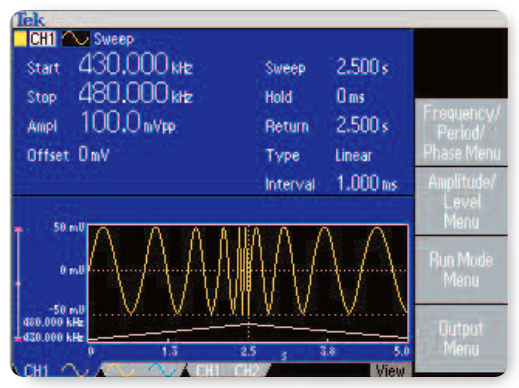
The AFG3252 simplifies the whole setup procedure by displaying related parameters such as start and stop frequencies, amplitude and sweep times in a single view. The next logical set of parameters is never more than one button-push away. In addition, the instrument displays an image of the waveform that will be produced, as shown in Figure 4.
Set Up The Acquisition and Capture the Waveform
On the oscilloscope, press "Acquire" and then choose "Peak Detect" by pressing the corresponding soft button. The Peak Detect mode will deliver an envelopestyle display that is easier to interpret than one made up of discrete waveform cycles.
The trigger settings are critical. The instrument evaluates the input signal and runs one acquisition (using the Single Sequence mode) to capture the data of interest,namely, one upward frequency sweep of the sine wave.The return sweep is ignored.
Press the "Trigger Menu" button and set the following parameters (Table 2).
| Type | Edge |
| Slope | Rising |
| Source | Ext |
| Mode | Single |
| Coupling | DC |
Table 2.
The trigger level is nominally 8 mV but this may need to be determined empirically for a given radio model. Next, set the Sec/Div to 250 ms and the input channel’s Volts/Div to 500 mV or an appropriate value determined empirically. With these settings you will capture and display an entire frequency sweep from 430 kHz to 480 kHz. Press Run/Stop to acquire the signal, and then position the trigger point, indicated by an arrow, at the far left side of the screen. In effect this places the 430 kHz end of the sweep at the left side of the display. Center the waveform envelope vertically before proceeding.
The result should be similar to that shown in Figure 5. The shape of this waveform envelope bears explaining. The input waveform contained frequencies from 430 kHz to 480 kHz. The envelope represents the IF amplifier’s inability (by design) to amplify all these frequencies equally. Frequencies significantly above and below the 455 kHz center point of the sweep fall off steadily to a lower amplitude than the specified intermediate frequency
Analyze the Results
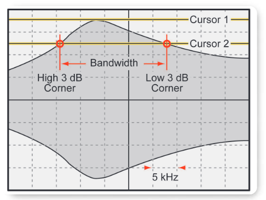
Looking at Figure 5, the bottom half of the waveform envelope is a mirror image of the information above the center line, and need not be considered in the analysis.
By convention the -3 dB point is defined as the frequency at which the signal’s amplitude is 70.7% of its peak value. Therefore the first step in calculating the bandwidth is to measure the peak amplitude. To do so, simply set a voltage Cursor 1 at the top of the envelope. The peak voltage value appears on the right-hand side of the screen. Multiply this value by .707 to obtain the - 3dB amplitude, and set voltage Cursor 2 to this value. The IF bandwidth is the span between the two points at which Cursor 2 intersects with the waveform envelope.
Because the full sweep encompasses a total of 50 kHz (430 kHz to 480 kHz) spread across ten horizontal time divisions, each graticule division corresponds to 5 kHz and each minor subdivision equals 1 kHz. Therefore the IF bandwidth can be calculated by counting the number of subdivisions between the points at which Cursor 2 intersects the waveform envelop and multiplying by 1 kHz. In this example the IF bandwidth of the AM section is about 23 kHz.
FM Section IF Bandwidth Measurement
The IF bandwidth measurement follows a procedure very similar to that of its counterpart in the AM radio section, although the frequency and amplitude parameters are different. In this example we will make a measurement on the First FM IF Amplifier. Figure 6 is a simplified schematic that focuses on the single NPN transistor comprising the active portion of the amplifier. Essentially we are measuring across the base-to-collector junction of this transistor. Of course, the surrounding capacitors and transformers play the major role in determining the net frequency response. The IF frequency of the FM radio section is 10.7 MHz. Ideally the bandwidth of the First FM IF Amplifier should fall within a range from 300 kHz to 500 kHz, but the actual result may depend on the quality invested in earlier setup steps such as AC gain, ratio detector alignment, etc.
The sweep function of the AFG is again used to simplify the characterization. The instrument sweeps automatically between two user-defined frequency endpoints; these must encompass a span greater than the expected bandwidth of the amplifier. The AFG settings in Table 1 are also appropriate for the FM IF measurements, although the frequencies must be changed to encompass the FM range. Because the IF bandwidth can appreciably exceed the ideal, it may be necessary to determine appropriate start and stop frequencies empirically.
–Start frequency: 10.1 MHz
-Stop frequency: 11.1 MHz
The oscilloscope’s Volts/Div setting should be 20 mV and the timebase setting should be appropriate for the frequencies involved. The TTL Out trigger from the AFG should be connected to the oscilloscope’s External Trigger input.
The remaining steps in the FM IF bandwidth measurement procedure are identical to those used in the AM section described earlier; refer to that discussion for details. In this case the frequency per division is 100 kHz rather than the 5 kHz value of the earlier measurement.
FM Section Final RF Alignment
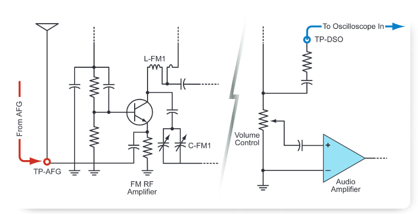
Connect the test equipment as shown in Figure 7. Note that this illustration encompasses two disparate sections of the radio: the antenna input with FM RF amplifier and the final FM section output to the audio amplifier. In effect we are connecting the signal source directly to the antenna, thereby simulating an FM broadcast.
| Modulation Type | FM |
| FM Source | Internal |
| FM Frequency | 1.000 kHz |
| Modulation Shape | Sine |
| Deviation | 22.500 kHz |
Table 2.
Set the AFG to a frequency of approximately 90 MHz (the low end of the FM band is 88 MHz) and an output amplitude of 50 mV.
Press the front-panel "Modulation" button to bring up a menu that controls internally-produced modulation formats that can be applied to the signal for each channel independently. Many signal sources require a second generator to add modulation but the AFG used in this application has a built-in modulation generator that simplifies this step. Table 3 summarizes the modulation settings that should be used.
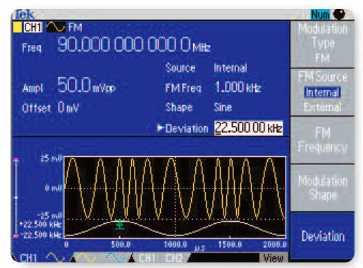
As before, all the settings are easily accessible with just a few button pushes on the front panel. A symbolic image of the waveform--including the modulation effect- -appears on-screen to confirm the instrument setting, as shown in Figure 8.
With the stimulus source connected, use the radio’s tuning dial to tune the reception frequency to 90 MHz or until the 1kHz tone becomes audible.
Set the oscilloscope to 200 mV/Div vertical gain; 500 microsecond horizontal sweep rate; 280 mV trigger level on the rising edge. The radio signal may be noisy; selecting HF Reject will abate this. AC coupling should be used.
Coil L-FM1 in Figure 7 is a variable inductor. The simplest way to determine and set its optimum value is to use two probing implements, one of brass and one made of iron. Each metal has a unique coupling response to the fields around the inductor. The interaction between the coil and the probing tools is the key to adjusting the reactive components (inductors and capacitors) in the radio’s input section.
First, place the brass tool near coil L-FM1. This will cause the coil to react as if inductance has been removed. Now observe the results on the oscilloscope. If the signal amplitude increases, the inductance of coil L-FM1 is too high and must be reduced.
Next, position the iron tool near L-FM1. This will cause the coil to react as if inductance has been added. Now monitor the oscilloscope waveform at TP-DSO. If the signal amplitude increases, in this case the inductance of coil L-FM1 is too low. Increase the inductance accordingly and repeat the "brass" and "iron" steps until the signal on the oscilloscope decreases in the presence of either metal.
Now increase the AFG carrier frequency to about 106 MHz, very close to the maximum frequency (108 MHz) in the FM band. Retune the radio until a 1 kHz tone becomes audible.
Position the brass tool near L-FM1. If the signal amplitude at TP-DSO increases, the capacitance of C-FM1 must be adjusted (increased). C-FM1 is a ganged dual capacitor that serves as the FM antenna trimmer.
Alternating the brass tool and the iron tool, follow the procedure used for the low-range FM adjustments described above, but adjusting C-FM1 instead of the coil. Repeat the test until the signal amplitude at TP-DSO decreases in the presence of either type of metal. Note that these adjustments affect the gain of the RF stage. As a whole the alignment ensures that the RF stage will track the FM oscillator stage correctly. It also has the effect of improving the alignment of the actual tuned-in frequency with the readings on the tuning dial.
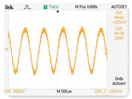
Figure 9 shows the oscilloscope display as it appears during this second, high-frequency part of the FM alignment procedure. This step illustrates the necessity for experimentation. To achieve the best results under the particular circumstances, the carrier frequency had to be set at 100 MHz and the input amplitude had to be increased. These measures were necessary to overcome interference from nearby broadcast stations. But the increased amplitude caused the amplifier stage to overdrive, which accounts for the slightly "flattened" tops on the sine waveforms in Figure 9.
Audio Performance of the FM Receiver
Ultimately the purpose of any consumer FM radio is to deliver audio to the listener. One final test will evaluate our example radio’s ability to do that. The audio frequency band is generally considered to encompass the range between 20 Hz and 20 kHz.
We will use the AFG to produce a sweep of frequencies as before, but with a difference. The audio performance test must use a full-frequency FM carrier that is modulated by an audio signal. This signal in turn is swept across the audio range. Using a single channel AFG, a second instrument would be needed to generate the swept audio signal. Thanks to the built-in second channel of the AFG3252, the swept audio signal can be generated with the same instrument as the FM carrier. The AFG and oscilloscope connections to the radio are the same as those in the FM alignment step just completed. The AFG and oscilloscope connections to each other are shown in Figure 10.
AFG Settings
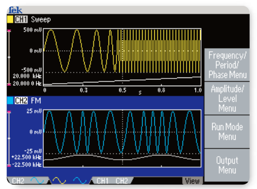
Figure 11 shows the AFG setup for this test. Channel 2 produces a carrier frequency of 100 MHz. Note that the modulation source is "External," unlike all the procedures explained earlier in this document. The deviation is set to 22.5 kHz.
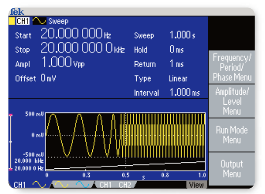
Channel 1 will generate the audio frequency and will use its internal sweep capability to vary the signal between 20 Hz and 20 kHz. Figure 12 depicts the setup for this signal. Important: note that the sweep time is set to 1 second. This is critical because you will need to listen for the sweeping audio signal when tuning to the carrier frequency. If the sweep time is too short, the sound of the individual sweep cycles becomes indistinguishable.
When two channels are used simultaneously, it is often helpful to view at a glance the settings affecting both channels. Figure 13 shows the summary screen for both channels used in this test.
The Channel 1 front-panel output must be physically connected to the rear-panel External Modulation input for Channel 2. A common 50-ohm BNC cable, one meter or less in length, serves the purpose. Both channels must of course be set to "ON" using their respective front-panel buttons.
Oscilloscope Settings
In an earlier measurement we used the oscilloscope’s Peak Detect mode, and that same method will aid the audio bandwidth measurement as well. Similarly, the Single Sequence feature makes it easy to acquire only the one sweep cycle needed for the test. The trigger must be set such that the instrument triggers at the same point near the beginning of each sweep cycle. If the swept audio signal is generated with Channel 1 of the AFG3252 as explained earlier, the Trigger Out signal of the AFG3252 can be used to trigger the oscilloscope directly, producing a very deterministic result. The AFG3252 Trigger Out is connected to the oscilloscope in the same manner as shown in Figure 3.
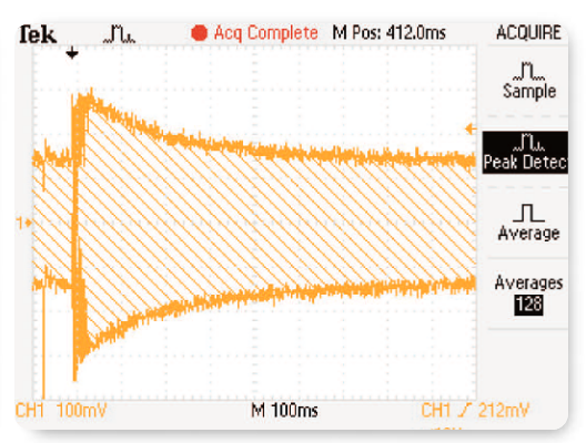
The overall audio performance of the radio can be interpreted from the Peak Detect waveform display using essentially the same technique explained in the IF Bandwidth section. Using a voltage cursor, determine the peak amplitude of the upper half of the envelope, then set a second cursor at .707 of that value. This is the -3 dB point. If the FM radio is designed for critical music listening, then the entire upper boundary of the waveform envelope should fall above the -3 dB cursor, all the way out to 20,000 Hz. If the radio is designed mainly for speech reception, then the response should taper off in the area above 3000 Hz.
Figure 14 implies that the example radio is in the latter category. Knowing that the audio sweep is linear, it is possible to estimate the frequency at any graticule division. Going from left to right, each of the 10 divisions represents a 2 kHz increase in frequency. Therefore the -3 dB point occurs at approximately two divisions after the peak. The bandwidth of the radio is about 4 kHz ideal for speech intelligibility without excess noise.
Conclusion
The task of setting up or troubleshooting an FM radio is made much easier with the help of a versatile signal source that offers the necessary frequency range (up to 108 MHz) as well as built-in modulation features. A multi-channel signal source can speed development of signals for tests including audio bandwidth, RF sensitivity, and IF alignment, Ease of use is another factor that appeals to radio designers, technicians, and service personnel. Fast access to frequently-used controls and menus means more productivity. And storable presets, too, can save time. A capable solution such as the Tektronix AFG3252 used in this document is a core tool in a host of AM and FM radio applications.
Find more valuable resources at TEK.COM
Copyright © Tektronix. All rights reserved. Tektronix products are covered by U.S. and foreign patents, issued and pending. Information in this publication supersedes that in all previously published material. Specification and price change privileges reserved. TEKTRONIX and TEK are registered trademarks of Tektronix, Inc. All other trade names referenced are the service marks, trademarks or registered trademarks of their respective companies.
12/06 75W-20333