Over the past decade, data communication rates have increased by a factor well over 10x. Data rates that were once 1 Gb/sec and below are now routinely greater than 10 Gb/sec. Optical communication is now routinely being designed at 100 Gb/sec and above, with research targeting 1 Tb/sec in the near future. RF wireless communications now employ broadband signals in the 20+ GHz range, and at the same time both RF and Optical Communications utilize complex modulation schemes and low amplitude signals to meet channel data capacity and regulatory requirements. This has driven the need for very high bandwidth real-time oscilloscopes for the validation, certification, and debugging of these new system designs. As a result, oscilloscope designers are driven to extend the performance of real-time oscilloscopes to cover requirements up into the 60 GHz-70 GHz range and beyond.
This document compares the techniques used to extend the bandwidth performance of real-time scopes, and introduces the latest innovation in this pursuit – Asynchronous Time Interleaving
The Conventional ADC Channel
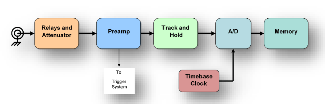
The conventional real-time digital oscilloscope channel typically employs an analog front-end, which normally consists of a preamp and/or attenuation for signal conditioning, and a track-and-hold for locking the signal amplitude during the sampling period. An analog-todigital converter (ADC) is used to convert the sequential voltage levels coming from the track-andhold to a stream of numeric values. See Figure 1.
Providing that the analog front-end supports the full bandwidth requirements of the channel, the sample rate of the ADC becomes the primary constraint to the bandwidth of the channel. The Nyquist Theorem states that in order to reproduce an accurate representation of all signal content within the desired bandwidth, the sample rate must be more than two times that bandwidth. For example, a 25 GHz channel bandwidth will require greater than 50 GS/s sample rate. As the bandwidth requirements continue to increase, finding ADCs that meet the Nyquist requirement becomes a bigger challenge.
It is appropriate at this point to consider channel noise for the conventional ADC channel, as this will become the foundation for further comments regarding channel noise associated with the techniques described on the following pages for extending the ADC performance.
Figure 2 depicts the random noise power spectral density (PSD) relative to frequency.

Because random noise by definition contains all frequencies, the PSD is spread equally across the Nyquist bandwidth of the instrument. In the case of a 50 GS/s channel, the Nyquist bandwidth is 25 GHz.
There is some noise rejection that occurs in Figure 2 because the scope BW limit filter (also called an anti-alias filter) rejects noise that exists in the spectral region between the cutoff of the BW limit filter and the Nyquist bandwidth of the channel.
Time-Interleaved Channels
As soon as the bandwidth requirements extend beyond the sample rate capability of the available ADC components, it becomes necessary to find other techniques to utilize available components to meet those extended requirements, or design a new generation ADC. Time interleaving is a common technique to extend the performance of existing components. Here, the analog front-end is designed to pass the entire bandwidth of interest, and two A/D converters are used in parallel. Each ADC must provide a sample rate at least half the total sample rate required to meet the Nyquist requirement. For example, provided that the analog front-end could support up to 45 GHz, two 50 GS/s A/D converters could be interleaved (see Figure 3) to provide 100 GS/s conversion. In this case, the two ADCs would be clocked 180o out of phase. Data would be stored in the memory behind each ADC, and once the acquisition completed, the entire 100GS/s representation of the waveform could be reconstructed by de-interleaving the data (sometimes called demuxing). It should be noted that there is not a limitation to how many ADCs can be interleaved, though it becomes difficult to carefully control the time alignment of interleaved devices as the ADC count goes up. This time-interleave technique has been used by all of the major oscilloscope manufacturers to get performance up into the GHz range.

It is important to note that as sample rate increases, the random noise is spread evenly across the new Nyquist bandwidth. In the example shown in Figure 4, the sample rate is increased from 50GS/s to 100GS/s, so the Nyquist bandwidth is now extended from 25 GHz to 50 GHz. If the noise performance of each of the time interleaved channels is equal, the noise power spectral density is now about half the power, spread evenly across the new Nyquist bandwidth. Of course, the goal in doing time interleave in this discussion is to extend the bandwidth of the system by providing a higher BW analog front-end, and a higher sample rate, but note that if the BW is kept to the same value as described initially (use the same scope BW limit filter), the net effect is to reject a larger amount of the noise signal.

Practical implementations of this approach have demonstrated noise reduction in the range of 15% - 20%.
Frequency Interleaved Channels - Mixing it Up with Downconverters
Downconverters have been used for well over a century in radio receivers and other RF applications. The concept is simple: mix two frequencies, and the result will be a sum and a difference in frequencies (also called heterodynes). If you can carefully select one of the two frequencies (e.g. a local oscillator) in relationship to the other, you have the ability to move the difference frequency to a more convenient range (typically lower) within which to work.
Using downconverters in conjunction with oscilloscopes is a technique that has also been used for a very long time. In the early days, the downconverter was an external unit, and the integration and calibration of the downconverter with the oscilloscope was left as an exercise for the user. Eventually, work was done to incorporate the downconverter into the instrument. In the case of an oscilloscope channel, setting the local oscillator frequency to equal the mid-band of the analog front-end bandwidth allows the possibility to acquire the upper half of the scope passband with one ADC, and the lower half of the passband with a another ADC. Reconstructing the total waveform by “stitching” together the upper and lower spectral halves becomes a DSP task within today’s digital real-time oscilloscopes.
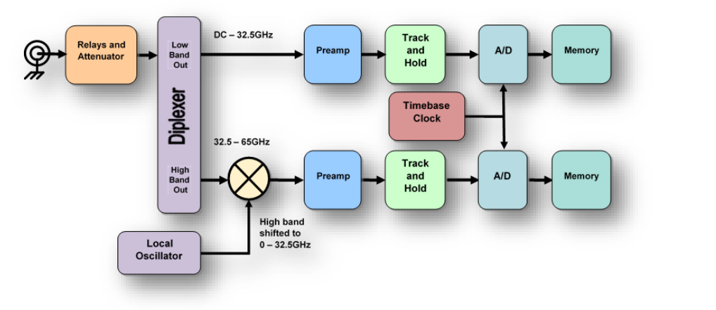
LeCroy was the first to implement this approach as an integrated capability in a digital scope, which they dubbed “Digital Bandwidth Interleaving” (DBI). Recently Keysight followed suit with their “RealEdge” channels. The key advantage for the oscilloscope designer is that each ADC needs only to have a sample rate that is greater than the total bandwidth. However, there are challenges in this design approach. Once the acquisition has completed, and the data is in waveform memory, it is necessary to up-convert the upper band back to its original frequency range using digital signal processing techniques (DSP). Recovering the two spectral “halves” and reconstructing the waveform is complicated. Because the paths are not identical, it is necessary to compensate for these differences in the calibration that is part of the DSP. Furthermore, due to the sharp cutoff of the bandpass filters used on the two spectral halves, recovering the exact center of the spectrum is problematic. We have seen issues with flatness at the recombination zone, as well as phase linearity shifts at that point.

Figure 6 shows an example frequency response plot for LeCroy’s LabMaster 10Zi-A 65GHz instrument, which uses DBI above 36 GHz bandwidth. Note that the frequency response is peaked up at the mid-band point, but has a distinctly different character in the range of 36GHz - 65GHz.
There is a similar problem with Keysight’s DSAZ634A instrument when using the “RealEdge” inputs. Figure 7 is a frequency response plot of that instrument. In general, Keysight has done a better job controlling the overall response compared to LeCroy, but notice the section of the plot at about 32 GHz. The mid-band crossover point is 31.5GHz, so it is not too surprising to see frequency interleaving artifacts in the range of 32GHz. The variation in amplitude at this area of approximately 1.3dB means that amplitude measurements of these frequencies will have an error of more than 15%.

Returning to the discussion of noise (Figure 8), it is informative to consider what happens to channel noise when using the frequency interleaving technique. As mentioned previously, the noise PSD is evenly spread across the Nyquist bandwidth (half the sample rate) of an acquisition channel. Because each ADC is acquiring half of the entire frequency span, there is no potential opportunity for noise reduction when going from Time Interleaved to Frequency Interleaved configurations (while keeping the bandwidth constant). In fact, there is generally a noise increase when using frequency interleaving. In Figure 9 a couple of screen captures demonstrate this on the Keysight DSAZ634A scope, comparing noise performance of a standard channel at 33 GHz bandwidth (screen on the left) to the noise performance of their “RealEdge” channel also at 33 GHz (screen on the right):

The Keysight scope measured baseline noise of 588µV rms on the standard channel, but measured baseline noise of 758µV rms on the "RealEdge" channel, with both measurements using 33 GHz bandwidth. The “RealEdge" channel has approximately 29% more noise than the standard channel with the same bandwidth. Granted, the above screen captures show the performance at the lowest gain setting (1mV/div), however even at a more typical setting of 20mV/div, the noise is approximately 18% higher on the RealEdge channel as compared to the standard channel for the same 33GHz bandwidth.

Asynchronous Time Interleaving – A Downconverter Technique with a Difference
In recognition of the technical issues and challenges involved with the architecture of the Frequency Interleaving that has been used to date in GHz bandwidth oscilloscopes, a new approach has been taken by Tektronix to avoid some of the disadvantages of DBI, while still accomplishing the end result of extended bandwidth with existing ADCs. With Asynchronous Time Interleaving (ATI), a pre-sampler is used as a harmonic mixer. Figure 10 illustrates the block diagram of the Asynchronous Time Interleave circuit:
One of the things that jumps out at first glance of this design is that the paths are symmetrical. There are no significant differences in propagation delay or phase shift between the two sides of the acquisition channel. This simplifies the post-acquisition process of DSP re-mixing or “reconstruction”, as compared with DBI, minimizing the amount of error at the mid-band crossover. With ATI, the entire bandwidth of the signal is applied to both ADCs. In this way, the power spectral density of the noise is evenly spread across the total sample rate, which is 2x the sample rate of the individual ADCs. The result is that the overall noise in the passband is lower than it would be in the comparable DBI architecture.

Because harmonic mixing and time sampling are really the same thing, it is possible to accomplish the mixing shown in the ATI circuit diagram (Figure 10) using a pre-sampler. This design utilizes the pre-sampler to intentionally sub-sample the input signal, thereby aliasing or folding back the upper half of the spectral content back into the Nyquist bandwidth of the ADC. For example, a 70 GHz system could be achieved by running the asynchronous sample clock at 75 GHz. This would result in the upper half of the 70 GHz signal being aliased back into the range of DC to 37.5 GHz. The resulting data from the pre-sampler could then be sampled by the ADC at a rate independent from the presampler, such as 100GS/s. Note that the pre-sampler is running asynchronously from the ADC sample clock. Figure 11 represents the signal on each leg of the ATI channel.


Figure 12 illustrates a more complete representation of the block diagram for the Asynchronous Time Interleave channel, with an indication of the spectral content of the signal at key points in the acquisition channel. As can be seen, the entire spectrum is applied to the preamp, and passes through the splitter to each pre-sampler. The output of the pre-sampler is a spectrum that contains a difference spectrum of the upper band folded back onto the lower band range, as well as the sum spectrum of the lower band overlaid on the upper band range. This complex spectrum is then passed through a low pass filter that removes the upper band range, but passes the lower band (including the folded back upper band content) intact. This filtered signal is then passed to the track and hold, and captured by the ADC.
Once the acquisition is complete, and the data is stored into memory, the original signal can be recovered by re-mixing the signal digitally using DSP techniques. At this point, rather than a physical Asynchronous Sampling Clock signal, a mathematical representation of that Asynchronous Sampling Clock signal can be used as input to the digital mixer, taking care that the phase relationship between the original analog Asynchronous Sampling Clock and the mathematical representation of that signal are identical.
Note that the two pre-samplers are 180o out of phase. This is important when it comes to reconstruction of the signal. After the digital mixing step of signal reconstruction, the numerical signal contains the sum and difference spectral content from the original acquired data. Conveniently, during the final combining of the signals, the portions of the spectrum that are 180o out of phase cancel, and all that is left is the original spectrum, plus a portion of the sum spectrum which is removed with a 75 GHz low pass filter. This leaves only the content from DC to 70 GHz that was originally applied to the scope for acquisition.
The final combining step is essentially a summation divided by two. This function returns the input amplitudes to their original value, but also has the effect of averaging the noise of the overall acquisition, thereby further reducing the total noise of the measurement channel.
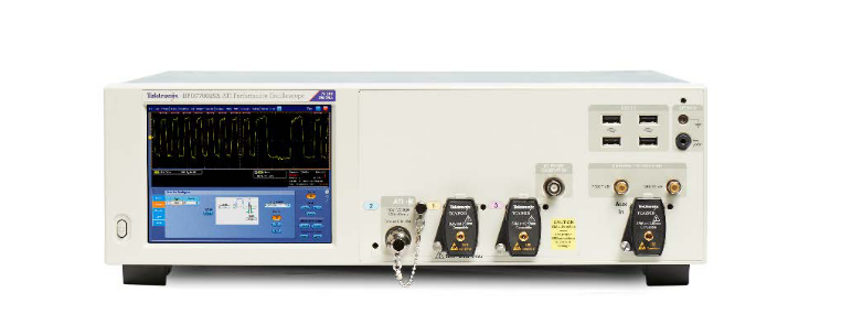
First ATI Implementation: DPO77002SX
Tektronix DPO77002SX 70 GHz ATI Performance Oscilloscope is the first production model incorporating ATI technology. It provides one channel at 70 GHz bandwidth, 200 GS/s using ATI technology or two channels at 33 GHz bandwidth, 100 GS/s using conventional real time acquisition.
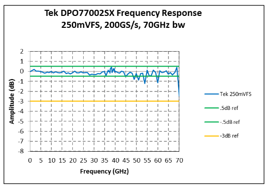
The frequency response of this new instrument demonstrates outstanding flatness out to 70GHz. As you can see in figure 13, there are no significant dips or peaking in the mid-band region. This assures the most accurate amplitude measurements across the spectrum.
Regarding noise performance, ATI again provides outstanding performance. Figure 14 shows a comparison of noise performance between a standard 33GHz channel and the ATI channel set to 33GHz bandwidth, with both set to the same vertical scale. We see here that rather than being higher noise on the ATI channel, the ATI channel is actually 21% lower noise. This is a significant contrast from the frequency interleave channels discussed previously. The left side screen shows the standard channel with a baseline noise of 1.05mV rms, while the right side screen shows the ATI channel with a baseline noise of 838uV rms.

The data shown in figure 15 demonstrates that ATI provides lower noise when compared to RealEdge. This is comparing the DPO77002SX against the DSAZ634A, with both scopes set to 60GHz bandwidth, maximum sample rate, and traces centered on screen. The plot shows measured baseline noise as a % of full scale. The ATI channel is as much as 30% lower noise than the RealEdge channel, depending on the full scale range selected.

In summary, Tektronix ATI technique provides:
- A superior method of extending the performance of existing ADC devices.
- Provides the highest signal fidelity.
- Maintains the lowest noise level.
The use of IBM's 9HP SiGe BiCMOS technology (with Ft = 300 GHz) provides the hardware performance necessary to realize a design to support a 70 GHz bandwidth target for a next-generation oscilloscope design.