Most power supplies and regulators are designed to maintain a constant voltage over a specified current range. To accomplish this goal, they are essentially amplifiers with a closed feedback loop. An ideal supply needs to respond quickly and maintain a constant output, but without excessive ringing or oscillation. Control loop measurements help to characterize how a power supply responds to changes in output load conditions.
Although frequency response analysis may be performed using dedicated equipment, newer oscilloscopes may be used to measure the response of a power supply control loop. Using an oscilloscope, signal source and automation software, measurements can be made quickly and presented as familiar Bode plots, making it easy to evaluate margins and compare circuit performance to models. A Bode plot maps the frequency response of the system through two graphs – a magnitude plot and a phase plot (phase shift in degrees). From these plots gain margins and phase margins can be determined to gauge power supply stability.
From this application note, you will learn:
- An overview of the basics of control loops, frequency response analysis and Bode plots
- A review of gain and phase margins
- How to set up control loop response analysis on an oscilloscope
- How to interpret frequency response plots and measurements
This application note uses a 5 Series MSO oscilloscope with Option 5-PWR Advanced Power Measurement and Analysis to demonstrate the principles of Bode Plots. The 4 Series MSO and 6 Series MSO have similar power analysis options with similar capabilities. The controls are very similar between these three instruments so this application note can be used to help understand the application of any of these three oscilloscopes in frequency response analysis.
Introduction to Frequency Response Analysis
The frequency response of a system is a frequency-dependent function that expresses how a reference signal (usually a sinusoidal waveform) of a particular frequency at the system input (excitation) is transferred through the system.
A generalized control loop is shown in Figure 1 in which a sinewave a(t) is applied to a system with transfer function G(s). After transients due to initial conditions have decayed away, the output b(t) becomes a sinewave but with a different magnitude B and relative phase ω. The magnitude and phase of the output b(t) are in fact related to the transfer function G(s) at the frequency (Ω rad/s) of the input sinusoid. The feedback coefficient ‘k’ determines how the input signal gets conditioned, based on the loads at the output.
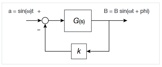
Here, B/A = |G(jω)| is the gain at ω, and Φ = ∠G(jω) is the phase at ω.
To understand the system behavior, the input sinusoidal signal is swept across range of frequencies at varying amplitude(s). This helps to represent the gain and phase shift of the loop taken over a range of frequencies and provides valuable information about the speed of the control loop and stability of the power supply. By sequentially measuring the gain and phase at various frequencies, a graph of gain and phase versus frequency can be plotted. By using logarithmic frequency scales the plots can cover very wide frequency ranges. These plots are often called Bode plots because of their use in control system design methods pioneered by Hendrik Wade Bode. Bode himself said, in his 1940 article in the Bell System Technical Journal, "Relations Between Attenuation and Phase in Feedback Amplifier Design":
The engineer who embarks upon the design of a feedback amplifier must be a creature of mixed emotions. On the one hand, he can rejoice in the improvements in the characteristics of the structure which feedback promises to secure him. On the other hand, he knows that unless he can finally adjust the phase and attenuations characteristics around the feedback loop so the amplifier will not spontaneously burst into uncontrollable singing, none of these advantages can actually be realized.
In power supply design, control loop measurements help to characterize how a power supply responds to changes in output load conditions, input voltage changes, temperature changes, etc. An ideal supply needs to respond quickly and maintain a constant output, but without excessive ringing or oscillation. This is usually achieved by controlling the fast switching of components (typically a MOSFET) between the supply and load. The longer the switch is on compared to the off time, the higher the power supplied to the load.
An unstable power supply or regulator can oscillate, resulting in very large apparent ripple at the bandwidth of the control loop. This oscillation may also cause EMI problems.
Gain Margin and Phase Margin
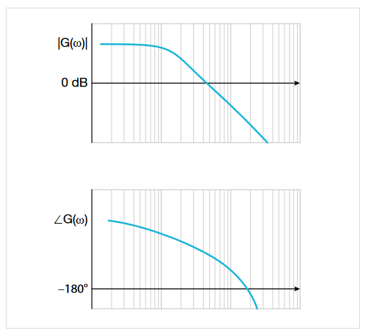
Instability will occur when the loop has positive gain (≥1) as phase shift approaches –180°. Under these conditions the loop will experience positive feedback and become unstable. Bode plots show gain and phase on the same frequency scale and let you see how close you are to this undesirable situation. Two measurements taken from a Bode plot gauge the safety margin in a power supply control loop: phase margin and gain margin.
As noted above, the Bode plot is made up of gain and phase plots versus frequency. The gain plot is computed over a specified swept band as:
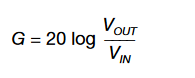
where VIN is a stimulus voltage applied to feedback of the control loop, and VOUT is the response of the loop at each of many points in the band.
The phase plot represents phase difference between VIN and VOUT at each frequency within the swept band. If the measured phase is more than 180°, then the plotted phase angle is measured phase –360°. If the measured phase is less than –180°, then plotted phase is measured phase +360°.
Phase and gain margin measurements are based on these plots. The formula for phase margin (PM) is:
PM = Φ – (–180°)
where Φ is the phase lag measured when gain is 0 dB.
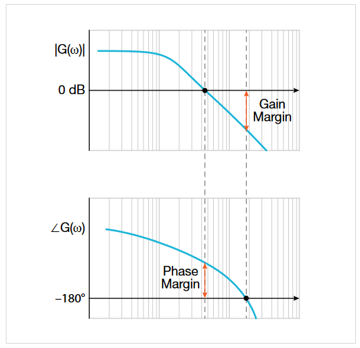
Phase margin (PM) indicates how far the system is from instability (–180° and unity gain) in terms of degrees of phase. It represents the amount of phase shift the loop can tolerate as the gain approaches 0 dB (unity gain). In other words, the phase margin describes the amount of phase shift which can be increased or decreased without making the system unstable. It is usually expressed in degrees. The greater the phase margin, the greater will be the stability of the system.
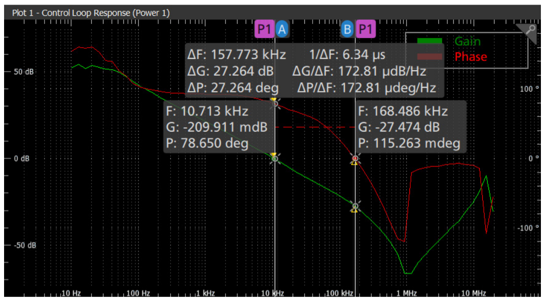
We can read the phase margin from the Bode plot by calculating the vertical distance between the phase curve (on the Bode phase plot) and the x-axis at the frequency where the Bode magnitude plot = 0 dB. This point is known as the gain crossover frequency. Gain margin is how far the system is from –180° and unity gain in terms of dB of gain. This is the amount of gain that could be added before hitting 0 dB, when phase shift = –180°. The gain margin describes the amount of gain, which can be increased or decreased without making the system unstable. The greater the gain margin (GM), the greater the stability of the system.
The gain margin (GM) is calculated by the formula:
GM = 0 – G dB
where G is the gain measured when the phase shift is 0°.
We can read the gain margin directly from the Bode plot by calculating the vertical distance between the magnitude curve (on the Bode magnitude plot) and the x-axis at the frequency where the Bode phase plot = 180°. This point is known as the phase crossover frequency. In the example shown in the graph above, the gain (G) at the crossover frequency is –20. Hence using our formula for gain margin, the gain margin is equal to 0 – (–20dB) = 20 dB and the loop is stable.
In short, maintaining ample phase and gain margin in the control loop ensures that a power supply will not operate too close to instability.
Oscilloscope Measurements using Automated Frequency Response Analysis
By measuring the actual gain and phase of the circuit over a range of frequencies, we can gain confidence in the stability of the design – greater than relying on simulation alone.
Performing a control loop response measurement requires the user to inject a stimulus over a range of frequencies into the feedback path of the control loop. Using an oscilloscope, signal source and automation software, measurements can be made quickly and presented as familiar Bode plots, making it easy to evaluate margins and compare circuit performance to models.
TEST SETUP FOR CONTROL LOOP RESPONSE MEASUREMENTS
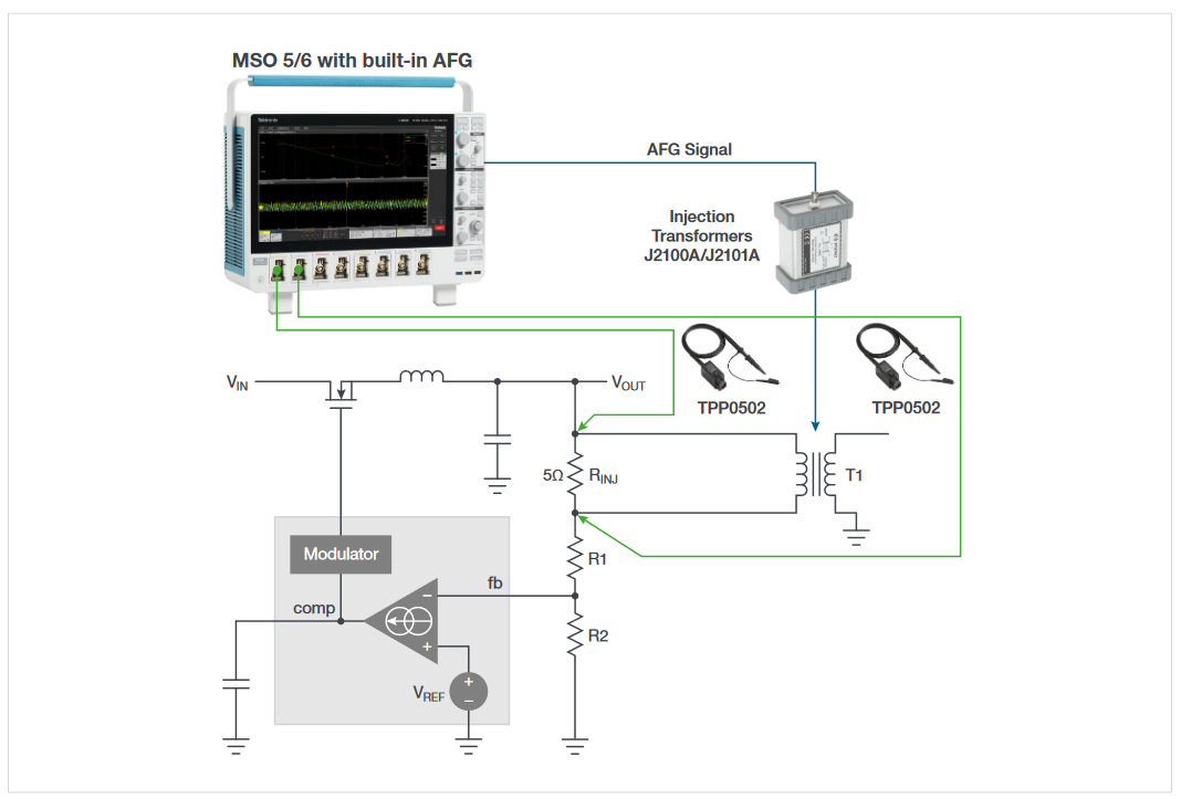
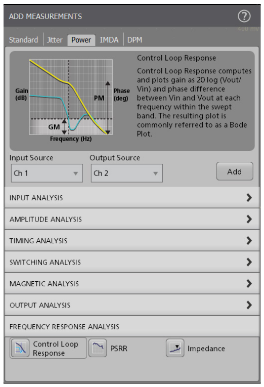
The 4, 5 or 6 Series MSO can be equipped with Advanced Power Measurement and Analysis software (4/5/6-PWR). This application software includes several frequency response measurements, including:
- Control loop response
- Power supply rejection ratio (PSRR)
- Impedance
For this application note, we focus on control loop response measurements. To determine the control loop measurements the analysis software performs the following important functions:
- Controls the function generator
- Calculates and plots gain (20 Log VOUT/VIN) based on the two voltage inputs, where VIN is the stimulus voltage from the function generator
- Calculates and plots phase shift between VIN and VOUT based on the two voltage inputs
- Calculates gain and phase margin
Two probes, applied across a low-value injection resistor, provide all the information the analysis software needs. It measures the stimulus and response amplitudes to calculate gain and measures the phase delay between stimulus and response.
To measure the response of a power system a known signal must be injected into the feedback loop. Several Tektronix oscilloscopes offer built-in signal sources that may be used to inject a signal into the loop’s feedback through an isolation transformer. For this example, the Arbitrary/Function Generator (AFG) option in the 5 Series is used to generate sinewaves over a specified range of frequencies. The DC-DC converter or LDO must be configured with a small (5–10 Ω) injection resistor/ termination resistor in its feedback loop so that a disturbance signal from the function generator may be injected into the loop. To avoid overdriving the control loop, the injection signal’s amplitude must be kept low.
An injection transformer with a flat response over a wide bandwidth is connected across the injection resistor and isolates the grounded signal source from the power supply. The choice of injection transformer depends on the frequencies of interest. The Picotest J2101A Injection Transformer has a range of 10 Hz–45 MHz which aligns well with the function generator option for the 4/5 Series MSO. Picotest also offers a J2100A Injection Transformer for use when frequencies are in the 1 Hz to 5 MHz range.
Low capacitance, low attenuation passive probes such as the TPP0502 are recommended for the voltage measurements. Low probe attenuation enables good sensitivity. The 2X attenuation of the TPP0502 enables measurements with vertical sensitivity of 500 µV/div on the 6 Series MSO, and 1 mV/div on the 4 or 5 Series MSO. Low capacitance of 12.7 pF minimizes probe loading effects.
MAKING FREQUENCY RESPONSE MEASUREMENTS
Once the DUT is properly connected, the stimulus sweep must be configured. Figure 6 shows the setup menu.
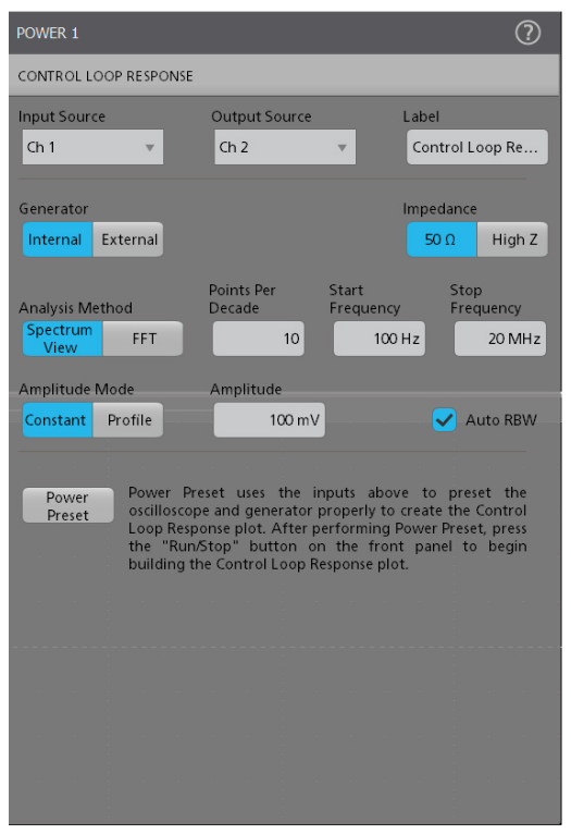
The number of points in the Bode plot are determined by the Points Per Decade, Start Frequency, and Stop Frequency.(The points per decade value is 10 by default, with a maximum of 100).
Number of frequency points is computed as:
Number of frequency points = ppd(log(fSTOP) – log(fstart))
For example, if the points per decade is 10, start frequency is 100 Hz and stop frequency is 10 MHz:
Number of frequency points = 10 (log(107) – log(102)) = 50 points
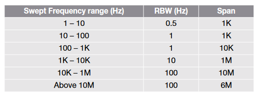
The Analysis Method refers to the method used for frequency response measurements. The default analysis method uses Spectrum View on the 4, 5 and 6 Series. This method uses digital downconverters built into each channel of these oscilloscopes. It provides flexible control over resolution bandwidth (RBW) and thus frequency resolution (typically mHz), compared to the traditional FFT method. The Spectrum View method is recommended, but the FFT method is still available as an alternative.
The Spectrum View method provides finer control of frequency resolution than the traditional FFT. The measurement setup includes the option of using “Auto RBW” (Figure 6) which helps take full advantage of this flexibility and resolution.
The Auto RBW control tells the instrument to automatically adjust key parameters of Spectrum View such as Resolution Bandwidth (RBW), Center Frequency (CF) and Span dynamically based on incrementally swept frequencies. This helps to balance RBW and Span across frequencies and provide stable and repeatable measurement results.
Table 1 shows how Auto RBW would adjust RBW and Span for optimal results for Bode plots from 1 Hz to above 10 MHz.
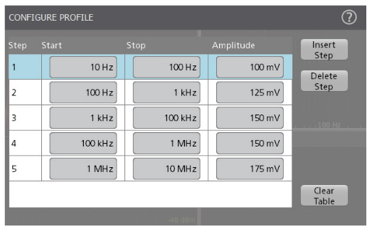
The 4/5/6-PWR software supports constant amplitude and profile amplitude sweeps.
- A constant amplitude sweep maintains the same amplitude at all frequencies. The start and stop frequency, amplitude and points-per-decade determine the sweep.
- A profile sweep allows you to specify different amplitudes at frequency bands you define. This allows you to improve the SNR (Signal to Noise Ratio). For example, you can test at lower amplitudes at frequencies where the DUT is sensitive to distortion, and test at higher amplitudes where it is less sensitive.
INTERPRETING THE RESULTS
To begin the test, one presses the front panel Run button.The measurement will start, and phase and gain curves will be plotted on the display. As soon as the green gain trace crosses the 0 dB line, phase margin will be displayed. When the red trace crosses the 0° threshold, the gain margin will be displayed.
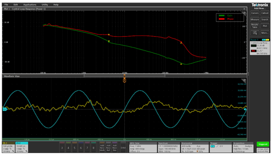
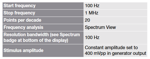
Figure 8 shows the gain and phase plots on a 5 Series MSO using the following settings to make measurements on a point-of-load regulator:
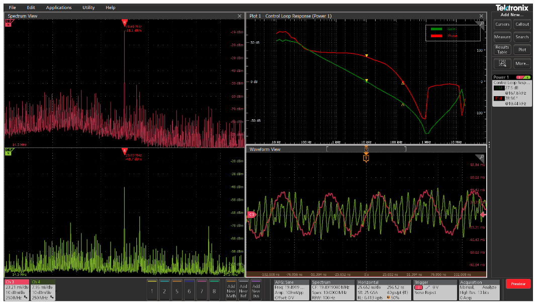
The resulting Bode plots and measurements show:
- Frequency on the x-axis, plotted on a logarithmic scale
- Gain (green trace) plotted on y-axis with the scale on the left. It is given in dB and is computed as 20 log (Vout / Vin).
- Phase between stimulus and response (red trace) is plotted y-axis with the scale on the right. It is given in degrees and plotted a linear scale.
- Spectrum View windows configured for input and output channels.
Gain and phase margins are presented in “badges” on the right. For the example shown in Figure 8, the gain margin measures 53 dB and phase margin measures 43°. As shown in Figure 10, cursors may be used on the Bode plots to indicate gain and phase at any frequency. The difference between the two cursors is also displayed. Being able to quickly pick off measurements helps accelerate debugging.
Summary
Most power supplies and voltage regulators are essentially amplifiers with a closed feedback loop. Control loop measurements help to make sure a power supply design responds to changes in output load conditions without excessive ringing or oscillation.
Frequency response analysis may be performed with dedicated equipment; however, newer oscilloscopes may be used to measure the response of a power supply control loop. The 4, 5 and 6 Series MSOs can be configured with built-in function generators further reducing the need for specialized equipment and eliminating the need for Frequency Response Analyzers or VNA's.
Using an oscilloscope, signal source and automated software, measurements can be made quickly and presented as familiar Bode plots making it easy to evaluate margins and compare circuit performance to models.