
This primer describes methods for making measurements using inverter, motor and drive analysis software on oscilloscopes to provide stable, accurate electrical measurements on the inputs, DC buses, and outputs of variable frequency drives, as well as mechanical measurements on the motor.
In this primer you will learn:
- Basic variable frequency drive structure
- Fundamentals of pulse width modulation (PWM)
- How to select and set up oscilloscope probes
- Selecting the proper wiring configuration
- How to make measurements on variable frequency drives
- – Electrical measurements
- Input Measurements
- DC Bus Measurements
- Output Measurements
- DQ0 Measurements
- – Mechanical Measurements
- Speed, Direction and Acceleration
- Torque
- Mechanical Power
- System Efficiency
- – Electrical measurements
This primer illustrates these measurements on a Tektronix 8-channel, 5 Series B MSO Oscilloscope, equipped with Inverter Motor Drive Analysis software which enables stable, accurate measurements on PWM waveforms.
Most modern motor drive systems use some form of modulation to control the frequency and therefore the speed of a motor. In most cases, these variable frequency drives (VFD) achieve this by outputting carefully controlled pulse-width modulated (PWM) waveforms. These systems typically output power as 3 phases since this is the optimal configuration for electric motors.
Three-phase AC induction motors (ACIMs) have been the workhorse of industry since the earliest days of electrical engineering. They are reliable, efficient, cost-effective and need little maintenance. However, there are a number of different types of motors and drives. AC induction motors (ACIM) are less efficient than Brushless DC motors (BLDC) and permanent magnet synchronous motors (PMSM).
Synchronous BLDCs and PMSMs are more efficient and lighter than AC induction motors but require more advanced control algorithms.
Although each type of system has unique characteristics, motor drives all use pulse-width modulation techniques to vary the frequency and voltage delivered to the motor.

Challenges in Making Motor Drive Measurements
Due to the pulse-width modulation on the output of motor drives, making stable measurements on these signals is challenging. Manually determining the right combination of filters and triggers to achieve stable waveforms is very difficult, yet this is a prerequisite for achieving consistent measurements.
In addition to measuring the output of the drive, measurements to evaluate the performance of the drive's input stages, such as harmonics, power and power factor are also important. While exporting raw waveforms into a spreadsheet or other analysis software is possible, the process is time-consuming and requires care in designing calculations.
These measurements involve many connections to the device under test. Incorrect probing of the motor drive system and poor integrity of connections are common sources of errors in making motor drive measurements.
Mechanical measurements are also key and can be made using sensors. However, it may be difficult or impossible to get measurements in engineering units of speed, acceleration or torque without custom processing and scaling.
For these reasons getting a good view of a motor drive system with an oscilloscope requires careful setup, stable waveforms and robust measurement algorithms.
Principles of PWM Motor Drives
Forms of pulse width modulation are used to drive many types of motors, including brushed DC motors, AC induction motors, brushless DC motors and permanent magnet synchronous motors. PWM allows the drive to vary the frequency and voltage delivered to the motor.
Although the principles of PWM drives have been understood for years, advances and cost reductions in power semiconductors, control electronics, and microprocessors have greatly stimulated the use of such drives. This has been further accelerated by vector control methods which enable designers to achieve the efficiency and controllability of DC motors with the reliability of AC motors. BLDCs and PMSMs are replacing brushed DC motors and AC induction motors in a wide range of applications including not only industrial applications but also power tools, appliances and electric vehicles.
A block diagram of the essential elements of a 3-phase Variable Frequency Drive is shown in Figure 2.

PWM drives can be powered by DC, single-phase AC, or 3-phase AC. Figure 2 shows a VFD powered by a 3-phase supply, which is common in industrial equipment. The 3-phase supply is rectified and filtered to produce a dc bus which powers the inverter section of the drive. The inverter consists of three pairs of semiconductor switches (MOSFET, GTO, power transistor, IGBT, etc.) with associated diodes. Each pair of switches provides the power output for one phase of the motor. This basic architecture can be adapted to serve several types of motors, however the control electronics vary greatly in terms of feedback and complexity. Here is a brief description of a few common forms of PWM used to drive motors.
6 Step / Trapezoidal Drives
This type of drive is used with BLDC motors. BLDC motors are efficient and small. They offer the benefits of DC motors, but they have no brushes to wear out. They can be electronically commutated with a relatively simple 6-step, or trapezoidal, PWM strategy. A typical set of PWM waveforms is shown below.

Scalar Drives
Simple VFDs used to drive AC induction motors control the speed by changing the fundamental frequency of the PWM waveform driving the motor. In order to maintain full torque, the control system in the drive maintains the ratio between the voltage and fundamental frequency of the PWM waveform. These are called scalar drives.
The control electronics generate three low-frequency sinewaves, 120° apart, which modulate the width of the pulses for each pair of switches.

The average voltage presented to the motor winding is approximately sinusoidal. The other two phases of the motor winding have similar average voltages spaced 120° apart.

To a large extent, the motor appears as an inductor to the output voltages of the inverter. As an inductor has higher impedances to higher frequencies, most of the current drawn by the motor is due to the lower frequency components in the PWM waveform output. This results in the current drawn by the motor being approximately sinusoidal in shape.

By controlling the amplitude and frequency of the modulating waveforms, and controlling the V/Hz ratio, the PWM drive can supply 3-phase power to drive the motor at a required speed.
Vector Drives / Field-Oriented Control
The more advanced drives for AC induction motors and synchronous motors employ vector drive techniques. These drives are more flexible and efficient than scalar drives, but also more complex.
Vector drives have similarities with scalar ones in that they drive the motor with sinusoidal current, however vector drives provide smoother operation, quicker acceleration, and superior torque control. These control systems often use field-oriented control (FOC) and are significantly more complex than scalar drives.
The vectors, D and Q are orthogonal vectors, whose magnitudes relate to the torque and magnetic flux within the motor.

The control system must measure the position of the rotor in order to synchronize the system. This is often done by using sensors such as Hall sensors or a quadrature encoder interface (QEI). (Sensorless systems are also used in which the control system uses the back-emf of the motor to determine rotor position.) The controller uses the Clarke and Park transform to calculate the magnitudes of D and Q, and then uses these values as setpoints for the control loop.

Making connections to a VFD system
Oscilloscope Probe Selection
Making power measurements on variable frequency drive systems requires voltage and current probes. When selecting oscilloscope voltage probes for motor drive measurements, it is important to consider:
- Motor drive measurements involve relatively high voltages. For example, the DC bus voltage in a 480 Vac three-phase motor drive is typically around 680 Vdc. Confirm the voltage rating at the probe tip and for the accessories used to connect the probe.
- Common-mode voltages can also be relatively high. That is, measurements are often "floating" relative to ground, so groundreferenced probes may not be used. It is important to be sure signals are not floating more than the common-mode voltage rating of the probe.
- Most frequencies of interest are below 200 MHz, so probes with this bandwidth should be sufficient for most everyday measurements.
- Probes should cover a wide range of measurement tasks.
For these reasons, high-voltage differential probes are generally recommended as general-purpose voltage probes for power electronics inverter subsystem, drive input/output, and control system measurements.

Note: Ground-referenced passive probes should not be used to measure phase-to-neutral voltages. The neutral terminal is robably not at ground potential, causing significant currents to flow through the probe and oscilloscope earth ground. This is dangerous and may result in shock or damage to the DUT or scope.

Some of the recommended probes for motor drive applications are:
| Model | Description |
| High-Voltage (Differential) Probes: THDP0100/0200 |
THDP Series probes are a good, general-purpose choice for making non-ground referenced, floating measurements on a wide variety of power electronics inverter and motor drive subsystems. They can perform measurements floating hundreds of volts above earth ground and measure differential voltages up to 6000 V, depending on the model. 100 MHz and 200 MHz models are available. |
| Optically Isolated Voltage Probes IsoVu TIVP Series: |
IsoVu probes offer extremely high common mode rejection. They are especially well-suited for making accurate high-side VGS measurements in switching circuits and are often used in validation of SiC and GaN applications. Various tips are available. MMCX tips deliver high signal integrity up to 250 V. Square pin tips are available in both a 0.100 in (2.54 mm) pitch that can be used in applications up to 600 V and a 0.200 in (5.08 mm) pitch that can be used in applications up to 2500 V. |
| Current Probes TCP0030A and TCP0150A |
AC/DC current measurement probes. The TCP0030A provides greater than 120 MHz of bandwidth with selectable 5 ARMS and 30 ARMS measurement ranges. For higher currents, the TCP0150A goes up to 150 ARMS. |
Oscilloscope Probe Setup
Before taking any power measurements, a few important steps must be taken. Current probes must be degaussed, and all probes should be de-skewed for accurate results.
It is important to perform a degauss procedure on current probes before taking measurements to remove any residual magnetization from the probe's magnetic core. Residual magnetization will cause incorrect measurements. The procedure is typically performed by removing all conductors from the jaw of the current probe and initiating the procedure with a button press. Tektronix current probes, such as the TCP0030A, will automatically prompt you to perform a degauss procedure before use.
The deskew process corrects for various propagation delays between any two different scope channels, including the probe and probe cabling. This is important since phase relationships are critical for many of the measurements on VFD systems. The basic procedure is to provide channels with a synchronized signal and adjust delays for each channel to align them. A power measurements deskew fixture (P/N 067-1686-xx) is available from Tektronix to help with this.
When connecting current probes, it is important to pay attention to the arrow on the probe. When the current probe is connected on the line side of the load, the arrow should point toward the load. If the current probe is connected on the return side of the load, the arrow should point away from the load.
For additional information on probe selection and setup for power measurements, see Probing Techniques for Accurate Voltage Measurements on Power Supplies with Oscilloscopes and Making Accurate Current Measurements on Power Supplies with Oscilloscopes.
Wiring Configurations
Often, both the input and output of VFDs use three phases. However, some VFDs used in commercial, residential, or automotive drive systems may be powered by single-phase AC or DC. In addition, 3-phase systems can be wired and modeled in two configurations: star (or wye) and delta. The wiring configuration determines the calculations used in power analysis, so it is important to understand and select the correct wiring configuration in order to get the expected results. These configurations apply to both the inputs and outputs of motor drives. Figure 11 shows wiring configurations supported by the IMDA solution on select Tektronix oscilloscopes.

Single-Phase Connections
1 Phase–2 Wire (1V1I)
Two channels are required: one for voltage and one for current, as shown in Figure 12, the voltage is measured.The total power measured, P = V*I. Single-phase AC and DC sources use the same setup.

1 Phase–3 Wire (2V2I)
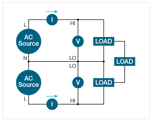
The 1 phase-3 wire configuration is rare in motor drive applications but is often found in North American residential applications, where one 240 V and two 120V supplies are available and may have different loads on each leg. Measuring such a source requires two voltage channels and two current channels. The total power measured is V*I (Load1 + Load2).
3-Phase Connections
Measuring 3-phase, 3-wire system with 2 voltage channels and 2 current channels (2V2I)
Motor drives often use 3-wire outputs which can be accurately measured by using just 2 voltage and 2 current channels on the oscilloscope. (Motor drive inputs are more likely to use a 4-wire system.) When three wires connect the source to the load, at least two wattmeters are required to measure total power. Two voltage channels and two current channels are needed, as shown in Figure 14. The voltage channels are connected from phase to phase, with one of the phases acting as a reference. The load and source can be wired in delta or star configurations but there must not be a neutral conductor between them. In this situation two wattmeters can account for the total power being delivered to the load. (See the sidebar: "How can 4 oscilloscope channels measure a 3-phase system?")

Figure 14 shows the wiring and Figure 16 shows the IMDA source setup for measuring a 2V2I connection. The Select Lines control establishes the phase used as a voltage reference. In this example the currents are measured on phases A and B, and voltages are measured on phases A and B with respect to phase C. That is, the measured values are VAC, VBC, IA, and IB. In this example, the total true power (ΣTrPwr) is:
The instantaneous power, P1 = VAC * IA
The instantaneous power, P2 = VBC * IB
ΣTrPwr = P1 + P2.
How can 4 oscilloscope channels measure a 3-phase system?
Blondel's theorem states that for an N-wire system, with voltage measured relative to one of the wires, total power can be measured using N–1 wattmeters.
For example, in a 3-wire system, either star or delta, the total power of the system can be determined by using 2 voltage channels and 2 current channels. For example, a star system is shown in Figure 15. Following Kirchoff's Current Law, all current in the system can be found if two of the currents are known. Voltages in the system can be determined by measuring two phases with respect to the third.

The instantaneous power measured by each wattmeter is the product of the instantaneous voltage and current samples.
Wattmeter 1 is comprised of iA and vAC, where
p1 = iA(vAC) = iA(v1 – v3)
Wattmeter 2 is comprised of iB and vBC, where
p2 = iB(vBC) = iB(v2 – v3)
p1 + p2 = iA(v1 – v3) + iB(v2 – v3) = iAv1 – iAv3 + iBv2 – iBv3
p1 + p2 = iAv1 + iBv2 – (iA + iB)v3 (Equation 1)
Per Kirchoff's Current Law,
iA + iB + iC = 0, so iA + iB = –iC (Equation 2)
Substituting for (iA + iB) in Equation 1:
p1 + p2 = iAv1 + iBv2 + iCv3 which is the total instantaneous power in all 3 phases.
Thus, the total power in the 3-wire system can be determined by using two voltage channels and two current channels to form two wattmeters.
Reference: Blondel, A.; Measurement of the Energy of Polyphase Currents; Proceedings of the International Electrical Congress; August 1893; American Institute of Electrical Engineers

Measuring 3-phase, 3-wire systems with 3 voltage channels and 3 current channels (3V3I)
Even though only two wattmeters are required to measure the total power in a three-wire system, there are advantages to using three wattmeters. The three-wattmeter configuration requires six oscilloscope channels: 3 voltages and 3 currents.
This 3V3I configuration provides individual phase-to-neutral voltages and the power in each individual phase, which is not available in the two-wattmeter configuration.

For 3-wire systems, measured with 3V3I, the IMDA software includes a setting to convert line-to-line (L-L) voltages to lineto-neutral (L-N) voltages. Although there is no physical neutral in this system, it is possible to determine the instantaneous line-to-neutral voltages from the instantaneous line-toline voltages.

This point-by-point LL-LN conversion expresses all voltages relative to a single reference and corrects the phase relationships between voltage and current for each phase. You can see the phase correction of the LL-LN conversion by noting the phase relationships on the phasor diagram with conversion turned on and off. Turning on LL-LN conversion allows instantaneous power calculations by multiplying phase-to-neutral voltages and phase currents. For example, we can find the total true power (STrPwr) being supplied to the load.
ΣTrPwr = (vAN * iA) + (vBN * iB) + (vCN * iC

Measuring 3-phase, 4-wire systems with 3 voltage channels and 3 current channels (3V3I)
Three voltage channels and three current channels are required to measure the total power in a system that uses a neutral conductor between the line and the drive, or the drive and the motor. Such a 4-wire system is shown in Figure 19. The voltages are all measured relative to the neutral. Phaseto-phase voltages can be accurately calculated from the phase-to-neutral voltage amplitudes and phases using vector mathematics. The total power, ΣTrPwr = P1 + P2 + P3.

Measurements for VFD System Blocks
Different measurements and techniques are used for different functional blocks within the VFD system. For each of these blocks (input, DC bus, output and motor) we will describe key measurements and note where they can be found in the IMDA analysis tools on the 5 and 6 Series MSOs.

3-Phase Autoset
The IMDA software includes a 3-phase Autoset function that automatically configures voltages and current sources based on the selected wiring configuration. It will optimally set up the vertical, horizontal, acquisition, and trigger parameters on the oscilloscope and may be done on all active power measurements. This greatly simplifies measurement setup, especially for PWM waveforms on the output of the VFD.
Input (line) measurements
Most industrial and heavy commercial VFDs have 3-phase inputs. Smaller drives may use single-phase line voltage. Especially in electric vehicle and other battery-powered applications, drives are often powered by DC. The IMDA power analysis software supports all of these configurations (see "Wiring Configurations") above. In the IMDA measurement package, the Power Quality and Harmonics groups are used to quantify the power consumption of the drive and the expected impact of the drive on a power distribution system.
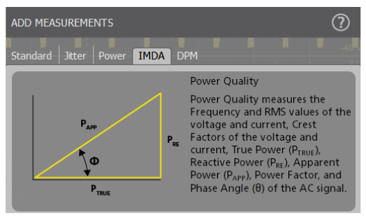
Power Quality
The Power Quality measurement group includes measurements that characterize the power consumption of the drive. These same measurements can be used on the output of the drive, as well (see "Output Measurements", below). Figure 21 shows the Power Quality measurement in the Electrical Analysis section. Selecting the Power Quality measurement produces a phasor diagram, waveforms and measurement badge. PQ Energy and Power math waveforms are shown for configured windings. The power waveforms are created using a math algorithm which multiplies voltage and current waveforms for each phase.
The Power Quality measurements are helpful for confirming that your probes and wiring configurations are correct. If one or more power measurements show negative readings,check your current probes – the ones on channels associated with negative power readings are connected backwards. For 3-phase systems, check the phasor diagram. Under normal circumstances, the voltages should be practically identical with 120° between the phases.
The user has the option to measure power quality for the fundamental or at all frequencies. When the fundamental frequency is selected, measurements will be only made on the fundamental frequency component. When the "all frequencies" option is selected, power quality measurements are computed for all harmonics including the fundamental frequency.
Phasor Diagram: The phasor diagram shown in Figure 22 is a circular diagram that represents magnitudes and phase angles between phase voltages and currents, as well as between voltage and current for each phase. Ideally, a balanced 3 phase has vectors equal in magnitude and out-ofphase with each other by exactly 120°.

The phasor diagram (Figure 22) gives the following measurements for each phase:
- RMS voltage and angle relative to the reference phase voltage (VaN in Figure 22)
- RMS current and angle relative to the reference phase voltage
- Phase between voltage and current
- Power factor
The Power Quality measurement badge, an example of which is shown in Figure 23, gives a number of measurements. In this example, the 3V3I configuration provides the following measaurements for each phase:
- VRMS: The RMS value of the phase voltages measured over an integral number of cycles. The number of phase voltages varies with wiring configuration.
- VMAG: The magnitude of the phase voltages measured at the motor operating frequency. The operating frequency is the fundamental frequency of the voltage signal and is determined by applying an FFT.
- IRMS: The RMS value of the phase current measured over an integral number of cycles. The number of currents can vary with wiring configuration.
- IMAG: The magnitude of the phase current signal measured at the motor operating frequency. The operating frequnecy is the fundamental freqeuncy of the current signal and is determined by applying an FFT.
- Crest factors (VCF and ICF): The ratio of peak voltage or current to RMS voltage or current. (The crest factor of a sine wave is 1.414.)
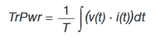
- True power (TrPwr): True power is given by
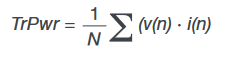
In the discrete domain this is:
where n = 1,2…N, and N is the number of samples.
True power (P) is the actual power delivered to the resistive part of the load, measured in Watts. Note that only for pure sinusoids does true power equal VRMS × IRMS × cos(ϕ), where ϕ is the angle between the voltage and current waveforms. - Apparent power (ApPwr) is:
where VRMS and IRMS are calculated from the voltage and current waveforms.
Units are VA.
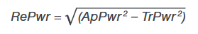
Note that performing an RMS calculation on the MATH1 power waveform is not equivalent and will not give the correct result. - Reactive Power (RePwr) is calculated as:
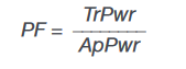
Units are VAR, or volt-amps reactive. - Power Factor (PF) is:
As the ratio of two powers, power factor is considered dimensionless. This calculation is preferable to using the cosine of the phase,
since it considers not only the fundamental frequency, but all measured frequency components. - Phase angle (Phase) is calculated as:
Units are degrees. As in the power factor calculation, this approach considers the full measured spectrum.


For any multi-phase system, the Power Quality measurement results give the following totals:
- Frequency (Freq) is calculated from the period of the lowpass filtered edge source.
- Sum true power (STrPwr) is the sum of the true power for all phases.
- Sum reactive power (SRePwr) is the sum of the reactive power for all phases.
- Sum apparent power (SApPwr) is the sum of the apparent power for all phases.

Harmonics
Harmonics measurements plot the signal amplitude at the fundamental frequency and its harmonics, and measures the RMS amplitude and Total Harmonic Distortion of the signal. Measurements can be evaluated against the IEEE-519 or IEC 61000-3-2 standard, or custom limits. For example, one can load limits for the IEC61000-3-12 standard as a csv file and test against these limits. Test results can be recorded in a detailed report indicating pass/fail status.

DC Bus Measurements
Ripple may be measured at two different test points, namely at the DC bus and on the switching semiconductors.
Line Ripple: This measurement provides the RMS and peak-to-peak measurements of the line frequency portion of the respective AC Voltage signals.
Switching Ripple: This measurement provides the RMS and peak-to-peak measurements of the respective voltage signals.

Switching analysis

When designing or validating the switching circuits within a VFD, it is important to understand the losses associated with the switching stages of the drive. Switching loss measurements and slew rates are available in Options 5-PWR and 6-PWR. Voltage probes are connected across the switch, and current probes are connected to measure current through the switch. You can add multiple measurements to get measurements for each switch.
The 5/6-PWR analysis packages include these measurements:
Switching Loss: measures the mean instantaneous power or energy in the turn-on, turn-off, and conduction regions of a switching device. The measurement creates a power waveform which is calculated for each pair of V and I waveforms.
dv/dt: measures the rate of change (slew rate) of the voltage, as it rises from the Base reference level (RB) to the Top reference level (RT), or as it falls from the Top reference level (RT) to the Base reference level (RB). The measurement creates a power waveform which is calculated for each pair of V and I waveforms.
di/dt: measures the rate of change (slew rate) of the current, as it rises from the Base reference level (RB) to the Top reference level (RT), or as it falls from the Top reference level (RT) to the Base reference level (RB). The measurement creates a power waveform which is calculated for each pair of V and I waveforms.
Direct Quadrature Zero (DQ0) transformations and measurements
Clarke and Park transformations are often used to simplify the implementation of field oriented control systems. An example of a field-oriented control system is shown in Figure 8. Within the control system, these tranformations are used to convert the 3-phase voltages being applied a motor to orthoganal D and Q vectors. These simplified vectors can easily be scaled and integrated to maintain a desired speed. Reverse transforms may then be used to create the drive signals for pulse width modulation in the inverter.
These D and Q vectors may reside deep within a digital signal processing block, such as an FPGA, and may not be available for direct measurement. The IMDA software offers optional DQ0 analysis that can derive measurements of D and Q based on the 3-phase output voltage or current with straightforward setup. This allows you to see the effect of control system adjustments quickly and easily.
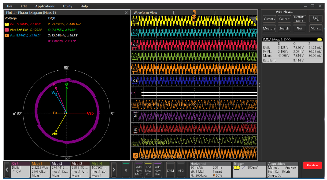
In addition to D and Q, the analysis software also shows the resultant vector (R). R is calculated by computing the D and Q hypotenuse vector at each of the sample points of D and Q. The R vector starts at 0 degrees, determined by the QEI index pulse (Z). The incremental angle is computed by the QEI based on the encoder's pulses per revolution (PPR) and the motor's pole pairs. By observing the R vector rotation one can see whether the control system is driving the motor smoothly. One can also observe the number of commutations — note the six distortion points in the R vector plot in Figure 27 above, corresponding to six commutation steps. Figure 28 shows an example of the source setup for DQ0 measurements. In addition to selecting the sources and wiring, you can also specify a low pass filter that can be applied to all sources, or only to the edge qualifier. This is useful for reducing noise due to EMI pickup and switching noise.

Output measurements
The output waveform of a PWM drive is complex, consisting of a mixture of high frequency components related to the carrier and components at lower frequency related to the fundamental frequency driving the motor. Making oscilloscope measurements on PWM waveforms can be challenging, since it can be difficult to achieve a stable trigger.

The difficulty occurs because the waveform is being modulated at low frequency. High frequency measurements, such as total rms voltage, total power etc, must therefore be made at high frequency but over an integral number of cycles of the low frequency component in the output waveform.
One of the main benefits of IMDA software is the ability to make stable measurements on PWM waveforms. It demodulates the PWM waveform on a channel you specify as an "edge qualifier" and extracts the envelope as a "math channel". This enables precise synchronization for measurements.
The same power quality and harmonics measurements that are used on the input to the VFD can also be used on the output of the drive to check voltage, current, phase, and power. These are detailed in the "Input Measurements" section of this primer. The same wiring configurations are available for both input and output measurements with the exception of the 1-Phase, 3-Wire configuration which is only available as an input.

Efficiency measurements
Efficiency measures the ratio of output power to input power for respective input and output V and I pairs. On 5 and 6 Series MSOs, the two-wattmeter method (V1*I1 and V2*I2) is used on both the input and output. This allows complete measurement of 3-phase input and output power to be made using 8 input channels, as shown in Figure 31.


Mechanical Measurements
Mechanical motor measurements, such as angular position, direction of rotation, speed, acceleration and torque provide important feedback to control systems. Different types of sensors are used for measuring mechanical parameters, depending on the type of motor and control system. Motor speed is commonly described as revolutions per minute (RPM), or the number of full rotations completed in one minute around a fixed axis. Acceleration is the rate of change of speed. Torque is the rotary force produced by a motor on its output shaft, usually measured in Newton meters (Nm) and foot-pounds(ft-lbs). Torque may be used to determine the mechanical power output of the motor. This, in turn, can be used with electrical power to calculate overall system efficiency.
Tektronix motor drive analysis software with Option 5/6-IMDAMECH supports these transducers:
- Hall effect sensors
- Quadrature encoders
- Resolvers
- Torque sensors
The software also supports torque measurement based on motor current for motors with a fixed torque constant.
Hall Effect Sensors

Hall effect sensors are used to provide position feedback to control systems. For example, they are used in BLDC motors to monitor rotor position to synchronize commutation. Their output may be used to calculate speed, acceleration, and direction. They produce pulse outputs proportional to speed and are often used in a trio.
The IMDA software can use Hall sensor outputs to plot motor speed and acceleration, as shown in Figure 36. To set up the measurement, indicate the number of pole pairs and gear ratio so the software can properly measure speed. You can use TPP1000 passive probes or high voltage differential probes, such as THDP0200 or THDP0100, depending on the motor output power and noise levels. On the 5 or 6 Series MSO you can also use TLP58 logic probes on any oscilloscope channel to measure the sensor output pulses. Using a logic probe on one of the FlexChannel inputs converts the input into 8 logic channels, allowing a single channel to support multiple Hall sensors. By comparing the motor rotation to speed measurements, you can validate that your connections are correct.

Mechanical speed is calculated from the time, in seconds, it takes for one revolution of the rotor. Speed is given in revolutions per minute (RPM).

where the difference between the stop time (tsp) and start time (tst) represents one mechanical revolution of the rotor. The number of pole pairs, specified as in Figure 36, determines how many electrical cycles make up each mechanical revolution. The gear ratio, G, may be used to account for any gearing between the rotor and output shaft of the motor.

Acceleration is rate of change of speed per unit time

The IMDA software uses the order of rising edges or the order of falling edges of the Hall sensor outputs to determine the motor's direction of rotation.
To measure direction the number of pole pairs must be specified. Consider a two-pole-pair motor as shown in Figure 37, in which A, B and C represent Hall sensor positions 120° apart. The north pole (N1) of the first rotor magnet crosses Hall sensor A at 0 degrees and outputs a rising edge. If the configured direction of rotation is clockwise (A-B-C) N1 will cross Hall sensor B next, at 120 degrees from Hall A. However, N2 is only 60 degrees away from Hall sensor C and will cross Hall C first. Thus, for a two-pole-pair motor, the pulse edge sequence will be A-C-B.
The IMDA software also validates the direction by comparing the first rising edge on Hall A sensor with the next edge after 120 degrees. For example, if the first rising edge is from Hall A and a rising edge of Hall B is observed at 120 degrees, then the rotor rotation sequence is determined to be A-B-C, clockwise in this example. If after 120 degrees a rising edge is observed on Hall C, the rotation is A-C-B or counter-clockwise.


Quadrature Encoder Interface (QEI)
The Quadrature Encoder Interface (QEI) consists of a slotted disc mounted on the rotating shaft, light sources (LEDs), and light receivers (phototransistors).

The number of slits in the disc determines the PPR (Pulses Per Revolution). The light from LEDs passing through the slits on the disc is transmitted to phototransistors and converted to pulse signals which are 90° out of phase.


where speed is measured in RPM, and PPR is the number of pulses per mechanical revolution. Dtn is the difference between a state transition, that is where an edge occurs on Ph A and then and edge occurs on Ph B. There are 4 state transitions for each pulse cycle of Ph A, so there are 4*PPR state transitions per revolution. The gear ratio (G) may be used to scale the speed to account for sensors that are geared up (G>1) or geared down (0<G<1).
The incremental angle (or resolution) of the encoder is:
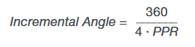
The IMDA software calculates the angle of rotation by counting the number of transitions and multiplying by the incremental angle.
Resolvers
A resolver is a type of sensor mounted on a motor to determine the angular position of the rotor. Due to its simple construction and reliability, it is widely used in rugged conditions with high temperatures and vibration. It consists of:
- An excitation coil that is driven by a high-frequency sinusoid input
- Two stationary orthogonal output coils

Figure 41 shows a block diagram of a resolver along with its output signals. It consists of a stationary part called the stator and a revolving part called the rotor, which is attached to the motor shaft.
The primary winding of the stator is connected to a highfrequency sinusoidal signal. This excitation signal is coupled by transformer action to a winding on the rotor. This rotor signal is the reference signal shown in Figure 42.
Two secondary stator windings provide the output signals. A sine and a cosine winding are mounted 90 degrees apart. As the motor rotates, the alternating magnetic field of the rotor winding induces an amplitude modulated voltage in the sine and cosine windings. The signal amplitudes at any given time depend on the angular position of the rotor. The relative magnitudes of the sine and cosine voltages may thus be used to determine the instantaneous angle of the rotor.
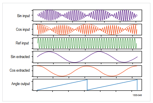
Mechanical measurements with a resolver require three analog input waveforms: sin, cos, and reference. The reference signal is the excitation signal, whereas the sin and cos signals are the output coil signals. The sin and cos signals are modulated by the reference signal. The sin and cos envelopes must be extracted in order to use them to make measurements. As expected, the envelopes, will have a phase difference of 90 degrees between them. At any given point in time, the motor's rotation angle is determined as:
Motor Angle = Arctan(ASIN/ACOS)
where ASIN and ACOS are the instantaneous voltages of the sin and cos envelopes.
Motor speed is determined by measuring the frequency of the sine envelope signal. For example, if there are two pole pairs, two cycles of the envelope represent one rotation.
Speed = Frequency(envelope signal)/pole pairs

Torque measurement
Motor torque is a rotary force produced by a motor on its output shaft. It is a twisting force measured in Newton meters (Nm), Foot-pounds (ft-lbs), ounce force-inch (ozf), Inchpounds-force (inch-lb), etc. The IMDA software on the 5/6 Series MSO supports two torque measurement methods.
Sensor Method
This is the most common torque measurement method, using a torque sensor or load cell output as shown in Figure 44. Measuring torque generated by motors can be done by coupling a rotary torque sensor in line with the motor shaft. One can capture the torque waveform using a passive voltage probe and the voltage waveform will be proportional to a measured torque value.

You must configure the high and low values of the torque sensor and the corresponding high and low values of the output voltage from the probe. The measurement will scale the acquired voltage waveform to torque values.
A load cell measures force. In this case torque is computed as product of force and arm length (distance) to convert the measured force to torque.
Current Method
Torque may be inferred from the RMS current in motors that have a specified torque constant. This provides an estimation of the torque value. Figure 45 shows the connection setup for torque measurements using the "Current Method".

In this case, the torque produced by the motor is directly proportional to the single or three-phase RMS current. The proportionality factor is represented by the torque constant of the motor.
Torque = Torque constant * IRMS
Mechanical power
Mechanical power generated at the output of a motor is computed as the product of measured speed and torque values. The multiplier is a constant used to provide mechanical power in watts. Speed is given in RPM. The value of the constant depends on the units used for torque measurements: 104.7252 for nm, 0.739522 for oz-inch, 141.9883 for ft-lb, or 11.83235897 for inch-lb.
Mechanical Power = (Torque * Multiplier) * Speed
System efficiency
System efficiency is the total efficiency of the motor drive system. It is also known as electro-mechanical efficiency. It indicates how much electrical energy is converted to mechanical energy. System efficiency is measured as the ratio of mechanical power from the motor to the three-phase electrical power used to supply the drive.
System Efficiency = Mechanical Power / Electrical Power

Dynamic Measurements
A common requirement in motor drive analysis is an ability to look at the motor response over time to monitor the DUT's behavior when accelerating and under varying load conditions. These dynamic measurements will help you understand the interdependency between parameters such as voltage, current, power and frequency under different conditions. The IMDA software offers two types of trend plots in the Power Quality measurement group to conduct this analysis:
- Time trend plots
- Acquisition trend plots
Each type of plot has its advantages and can be used to plot the supported sub-measurements within the Power Quality measurement group. The plots can be saved as a CSV file for post-processing.
Time trend plots
The time trend plot shows the measured value for each waveform cycle over a single acquisition. This is useful for examining and correlating detailed, short-term variations in measurements.

Acquisition trend plots
Acquisition trend plots record a single mean measurement value for each acquisition. This makes them useful for longer-term analysis. You can specify the test duration by setting an acquisition during the test configuration. The plots can be saved as a CSV file for post-processing. Time values are available when plot data is saved as a CSV file.
Dynamic load control is important for 3-phase induction motors and other electric motors as well. Acquisition trend plots make it possible to observe measurements during acceleration, at constant speed and during deceleration.

Summary
Making measurements on 3-phase motor drives presents challenges due to the connections that must be made, the complexity of waveforms and the daunting amount of math. IMDA software on Tektronix 5/6 Series MSO oscilloscopes greatly facilitates these measurements, providing power analyzer measurements with the benefits of the highspeed sampling systems and visualizations of real-time oscilloscopes.
With oscilloscopes, 3-phase motor drive designers can perform analysis under both static and dynamic operating conditions, observing both electrical and mechanical parameters for a thorough understanding drive performance. The sampling and processing power in the 5 and 6 Series MSOs enable capabilities such as DQ0 measurements that enable one to see deep inside control systems. These capabilities are not currently achievable with power analyzers.
Find more valuable resources at TEK.COM
Copyright © Tektronix. All rights reserved. Tektronix products are covered by U.S. and foreign patents, issued and pending. Information in this publication supersedes that in all previously published material. Specification and price change privileges reserved. TEKTRONIX and TEK are registered trademarks of Tektronix, Inc. All other trade names referenced are the service marks, trademarks or registered trademarks of their respective companies.
05/2023 48W-73863-1