A real-time spectrum analyzer (RSA) offers a lot of different measurement capabilities, including modulation and time domain analysis, pulse analysis and live real-time spectrum analysis. First and foremost though, it is a spectrum analyzer. There are differences in the way that an RSA generates spectrum results compared to a conventional swept spectrum analyzer. This note describes the spectrum processing that occurs in the RSA.
The architecture of an RSA is similar to a Vector Signal Analyzer, where the RF input is down-converted into a wideband IF stage where the IF signal is sampled and ultimately converted into quadrature (IQ) samples vs. time. All of the measurement displays, including the spectrum display, are computed from this IQ sample stream. If the measurement span is greater than the IF bandwidth, then the spectrum is computed in several segments.
Many vector signal analyzers perform this calculation using a Fast Fourier Transform (FFT). An FFT is computationally efficient, but places constraints on the vector length and the resulting frequency resolution (bin resolution). The spectrum computation in the RSA is performed using a Chirp-Z Transform (CZT). The CZT algorithm removes the constraints imposed by the FFT, giving the user full flexibility in selecting frequency span, resolution bandwidth and number of trace points.
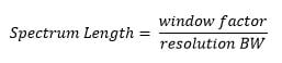
Spectrum results are computed by passing a time-seamless vector of IQ samples to the CZT. The vector is weighted by a user defined window function (default is Kaiser) prior to the CZT computation. The length of the vector in time (called the spectrum length) is determined by the window function being used, and the resolution bandwidth that is chosen by the user. Each window type has a “window factor” which affects the resulting spectrum length. The relationship is:

Some of the windows available in the RSA, and their -3dB window factors are (except for -6dB MIL window):
|
Window |
Window Factor |
|
Kaiser (default) |
2.2292 |
|
-6dB MIL |
2.9405 |
|
Blackman Harris 4B |
1.900 |
|
Flat-top |
3.720 |
|
Hanning |
1.440 |
The actual Spectrum Length shown in the Time Overview display becomes slightly larger than the above formula due to some rounding up to the required number of samples for processing, thus using a Resolution BW of 1MHz and a Kaiser window results in a Spectrum Length of 2.235μS instead of 2.2292μS.
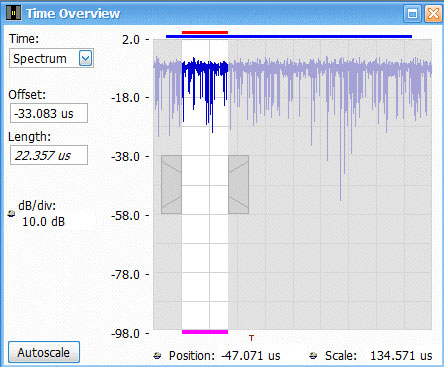
Given that the spectrum result comes from a time-domain vector of IQ data, the RSA gives you the ability to control the location of this IQ vector within a given RF acquisition. The Time Overview display allows you to visually see and control the spectrum vector position/offset with respect to the amplitude (vs. time) of the acquired RF signal. The red bar along the top of the display visually depicts the spectrum length. The user can adjust the Offset value to position the spectrum measurement where desired. Notice that the Spectrum Length of 22.357μS is italicized. This indicates that this value is automatically coupled to, and set by the RBW and window settings. In this case, the RBW is set to 100kHz with a Kaiser (default) window. The spectrum result is shown in the Spectrum Display shown below.

The result of the CZT computation is then sent through the user selected Trace Detector before being displayed. There are several available detectors, some of which are only available on certain RSA hardware. The most common detectors include +Peak, -Peak, Average (VRMS), and Sample. These detectors determine how the trace points are computed from the CZT result whenever there are more samples in the CZT result than the number of trace points.

In some cases, the number of trace points is equal to the number of samples produced by the CZT result (this may happen when the RBW is a relatively large fraction of the span, such as span/200). At lower RBW settings, the number of trace points can be increased to keep the CZT points equal to trace points. When this happens, the spectrum result will be the same for all of the Trace Detector types. In the Spectrum Display at right, you can see from the Trace Legend that there are three traces enabled with three different detector types, but each of these traces perfectly overlaps, so it looks like there is only one trace. Another benefit of the CZT algorithm is that increasing the number of trace points doesn’t dramatically increase the processing time. For example, increasing the the number of trace points from 801 to 64001 will typically result in <<2x increase in processing time.
There are typically two circumstances where the number of samples in the CZT result exceeds the number of trace points. One is where a very narrow RBW is selected along with a small number of trace points. The more common circumstance would be when the user adjusts the Spectrum Length to be greater than the auto-coupled spectrum length. This can be done by simply changing the Spectrum Length in the Time Overview display, or by linking the Spectrum Length to the Analysis Length. Once the Spectrum Length is >2x longer than the auto-coupled length, then multiple CZT results will be computed. The RSA will compute as many integer number of CZT results that will fit consecutively within the user selected Spectrum Length. For example, if the Spectrum Length is increased to 100µS for the acquisition shown, the RSA will compute four CZT results because that is the largest integer number of consecutive 22.357µS that will fit within the requested 100µS length.

The Spectrum Display now shows three different traces for the three different detector types. These traces reflect the result of applying the selected trace detector across all four CZT results obtained within the 100 µS spectrum length. Note that the pink bar along the bottom of the Time Overview display shows the region where the displayed spectrum results were computed. The pink bar accurately portrays the fact that the four consecutive 22.357µS CZT vectors don’t quite occupy the 100µS spectrum length.
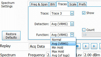
The Trace Detector selection applies to the processing of the CZT result to the displayed trace, for any given acquisition. Thus, it applies even to a single RF acquisition and analysis. The Trace Function applies to how the traces are processed over multiple acquisitions. The available trace functions are: Normal, Min Hold, Max Hold and Avg (of logs). As subsequent acquisitions are completed, the traces from each acquisition are combined with the previous traces using the selected function. For example, a Max Hold function will update the trace after each acquisition such that it reflects the highest recorded amplitude at each point on the trace from all of the processed acquisitions.
To summarize, the trace detector applies to trace processing within each acquisition, and the detector applies to trace processing across multiple acquisitions.
The ability to control the location of the spectrum computations within a seamless RF acquisition, as well as controlling the number of spectrum computations and the detector used, give the user a lot of power and flexibility to analyze and understand the spectral content of modern, transient and time varying RF signals.