
Modern radar signals make use of intra-pulse modulation or modulation on pulse (MOP), such as a linear frequency modulation (LFM), or some form of phase modulation (such as a bi-phase Barker code) to improve range resolution. They also include modulation on pulse to occupy more bandwidth and thus decrease the probability of intercept (POI). Additionally, intra-pulse modulation can include some form of communication or data transfer, such as in Secondary Surveillance Radar (SSR) of Identification Friend or Foe (IFF) systems. These employ various MOP techniques such as frequency or phase shift keying (FSK or PSK). Other LPI techniques include inter-pulse modulation, such as pulse-to-pulse frequency hopping.
Although these techniques bring significant benefits to radar systems, they also introduce new measurement challenges and requirements. Test and measurement instruments must have wide acquisition bandwidth and vector signal analysis in both the time and frequency domains. This allows radar engineers and researchers to look at both the scalar properties of the pulse (rise and fall times, pulse width, pulse repetition, and other time-domain characteristics) as well as the vector or modulation properties of the pulse and pulse train (frequency and phase deviation within pulses and from pulse to pulse, as well as modulation analysis of the intra-pulse modulation technique).
In this short post, we’ll explore how Tektronix software running on real-time spectrum analyzers and wideband oscilloscopes can help you make the following four measurements of radar signals:
- Amplitude vs. Time
- Phase vs. Time
- Frequency vs. Time
- More complex modulation schemes such as BPSK, QPSK, QAM, etc.
- Amplitude vs. Time
Rise time and fall time measurements have two different definitions. Many measurements use 10% to 90% of full amplitude as the definition of the transition time, but in some cases the definition is 20% to 80%. Tektronix SignalVu software allows the user to select either, as depicted here:

These points are defined as voltage points on the pulse waveform. However, even this much flexibility on definition is not quite enough. How one determines the top of a pulse can greatly affect the definition of transition time. If the top of the pulse is flat, then there is no problem calculating the pulse duration based on the signal power exceeding certain thresholds. However, if the top of the pulse is tilted or has droop, then the software could miscalculate the fall time. Let’s suppose that the pulse droops down by 20% over the duration of the pulse. The upper transition point is 90% of the highest part of the top, so the software will report the correct rise time. However, the fall time will be quite incorrect as the "falling" 90% point will be somewhere in the middle of the pulse due to pulse droop. SignalVu includes a compensation selection for this.
Figure 1. 50% level definitions
There are two standards available for the definition of the "50% point" of the pulse waveform. Baseband pulse measurements generally assume that the beginning and end of a pulse is the 50% point of the voltage waveform (Figure 1). However, measurements made on RF modulated pulses sometimes assume that the 50% point is stated in RF power, not voltage. SignalVu software gives users a selection of which of these definitions to use for the start point and stop point of pulses (Figure 2). These settings affect the measurements of width, period, frequency deviation and error, phase deviation and error, ripple, droop, ON power, and pulse-to-pulse phase and frequency.
Figure 2. SignalVu capturing a pulse and displaying rise and fall times
- Phase vs. Time
In a simple phase vs. time plot, the phase reference is the beginning of the acquisition record. Using this reference, SignalVu software plots the phase vs. sample number (expressed in time).
In Figure 3, the right side shows the frequency vs. time plot and the left side is the phase vs. time plot for the same acquisition. The signal is a single pulse with Barker-coded phase modulation. The phase plot shows various phase segments within the pulse. Note that for this code the phase values remain the same between segments one and two, and again between segments three and four, giving the appearance that two of the segments are twice as wide as the others.
Figure 3. The right side shows the frequency vs. time plot, and the left side is the phase vs. time plot for the same acquisition.
The frequency plot shows very large frequency glitches because the phase modulation has two problems. The first is that the segments inherently are not phase continuous. This has no impact on the phase plot but causes a large instantaneous frequency modulation at the instant of phase change. Such a discontinuity is a very short-term wide band spectrum "splatter" which may exceed the allowable spectrum mask for a very short time, may cause interference to equipment operating on nearby frequencies, or even create a recognizable "signature" for this radar system.
The second issue is that there is apparently little or no bandwidth limiting filter on this transmitter. This exacerbates these same phase discontinuities. If this were filtered, the frequency plot would be flat.
For the phase vs. time plot it is important to realize that since the phase reference is the beginning of the acquisition record, if the record starts within a pulse (triggered) then the phase may be similar from one acquisition to another. But if the beginning of the record is random, then the phase reference point is in the inter-pulse noise. This will result in a large random variation in the phase reference from one acquisition to another.
- Frequency vs.Time
The Frequency vs. Time display can measure the frequency of any single incoming signal including pulses. Like any FM detector, it will measure the combination of all signals within its detection bandwidth, so users should limit the capture bandwidth of the instrument to exclude any signals other than the one they are looking at.
SignalVu software computes the frequency versus time by measuring the phase at each sample and then dividing the phase change between two adjacent samples by the time between these same samples as "f = ∆ Ø / ∆t". Figure 4 shows a plot of the frequency change from one sample to the next with the horizontal axis in time for the user's convenience. It is important to note that since this is simply phase change versus time, no reference is needed (other than the main instrument time base) and the frequency plot is in absolute frequency.
Figure 4. A plot of the frequency change from one sample to the next
- General Purpose Modulation Measurements
The analysis of digitally modulated signals introduces greater complexity because the measurements include the amplitude and phase of the pulse plotted against specific, discrete combinations of amplitude and phase (symbols). These measurements many times require that the user enters the modulation type, symbol rate and the measurement and reference filter parameters as in the Figure 5.
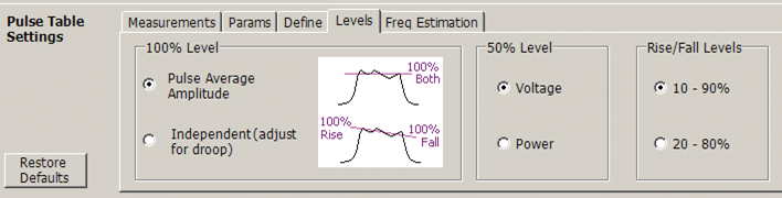
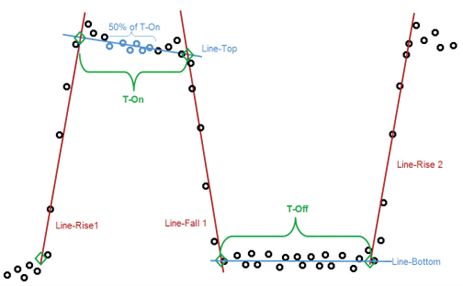
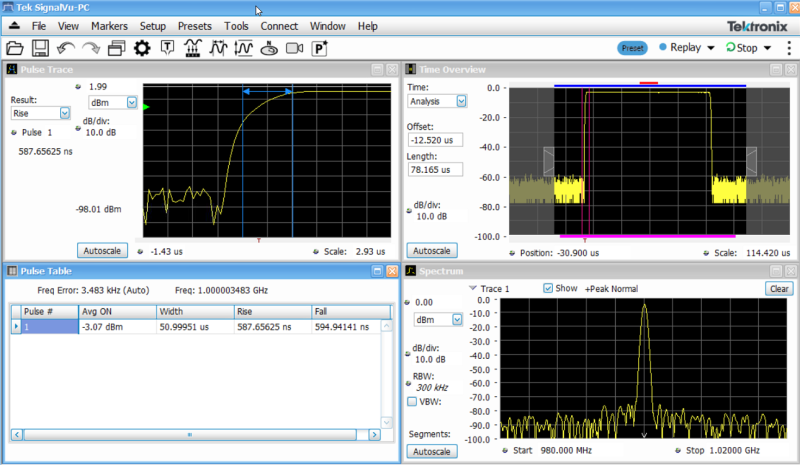
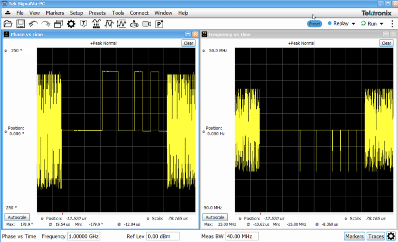
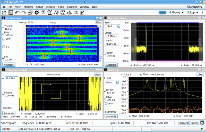
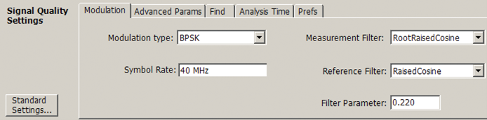
Figure 5. Analysis of digitally modulated signals requires entering the modulation type, symbol rate and the measurement and reference filter parameters.
The instrument can then more accurately perform the measurement and display the symbol constellation, error plots, signal quality and a demodulated symbol table. Figure 6 shows a constellation display of a higher-order QAM pulse on the left and both signal quality and a spectrum plot on the right.
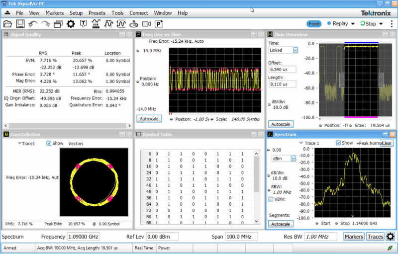
Figure 6. A constellation display of a higher-order QAM pulse on the left and both signal quality and a spectrum plot on the right.
Tektronix provides a broad selection of test equipment suitable for radar pulses. There are instruments with specialized pulse measurements and measurement bandwidths up to 70 GHz, and signal generation equipment with radar pulse synthesis capability to near 15 GHz of instantaneous bandwidth.
For more information on pulse measurement methods, download the full primer – Fundamentals of Radar Measurements.