
By Josh Brown
Transient recovery time, simply put, is duration of time needed for a power supply to return to its set level after a load is applied. Those of us who do not design power supplies have a tendency to take this for granted, applying whatever loading circuitry we are working on until, perhaps, the supply performance degrades to the point it impacts our own work. Power supplies are a little like people, if you ask more from them than they are capable of, they won’t perform like you might expect.
Let’s use an analogy to help illustrate the importance of accounting for power supply stress. If someone tosses you a baseball and tells you that when you catch it the ball needs to stay at the same height, give or take a few inches (or centimeters) and get there within 1 second. The baseball (the load) is relatively light and when you catch it, your hands barely move. (Provided, of course, that you have an accurate pitcher.)
Now imagine someone tossing you a bowling ball and imposing the same restrictions on your response. Not only do your hands move but also your body moves to help due to the weight change. Did the ball cause the height you are holding it at change with respect to the target height? How much? Could you catch and hold the ball at all? If you were able to keep it within a certain height tolerance, were you able to stabilize your height within the 1 second interval allowed? Obviously, this is a far tougher challenge (unless perhaps you're an NFL lineman), and similarly if the load you place on the power supply is more than it can handle, it will struggle to meet your requests.
But how do you know when you’ve gone too far? That’s where thorough characterization of transient recovery characteristics with a DMM is key.
Before diving into the specifics, we should first discuss switching frequency, as this will help determine the instrument you choose for evaluating the behavior in question. While both linear and switch mode power supplies are subject to transient recovery time specifications, the latter operates with a predetermined frequency, naturally has more noise and is subject to some more spurious signal activity. The frequency range used by switched supplies is typically from 10 kHz to 1 MHz. Because oscilloscopes have high sampling rates and are great visual tools, they are ideal for evaluating transient recovery time using level triggering for event capture and on-screen cursors for math and measurement analysis.
A digital multimeter with a high-speed sampling function is something you may also want to consider and may already be available on your bench. Some DMM models have been able to sample up to 50 kHz for many years and newer models are capable of rates up to 1 MHz. With the speed comes more opportunities for high-speed sampling with greater measurement sensitivity than most oscilloscopes.
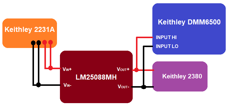
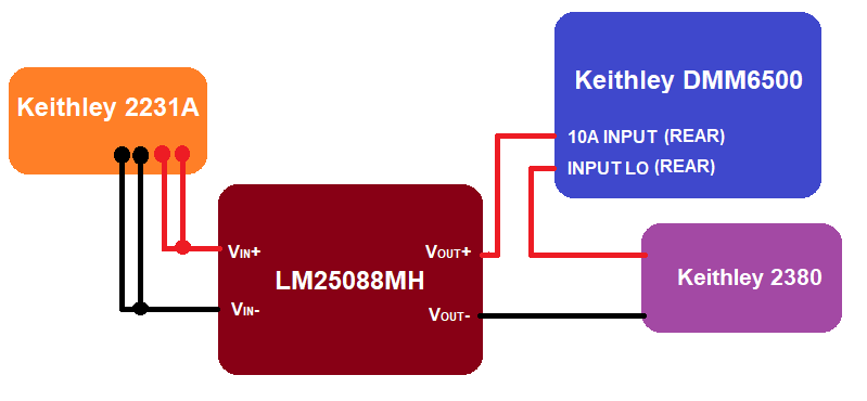
As an example of how to measure transient recovery time, we use the LM25088MH-1EVL evaluation board from Texas Instruments which is capable of supplying 5V at up to 7A from an input supply of up to 36V. With some minor modifications, we have reconfigured the unit to switch at 25 kHz. We use two channels of a Keithley 2230A-30-3 Triple Channel DC Power Supply to provide a 10V input signal with up to 6A of current to power the evaluation board. We also use a Keithley 2380-500-15 electronic load to sink a specific amount of current. In this case we want to push the LM25088MH to its 7A limit to see how it responds. We will use a DMM6500 to first evaluate the voltage response to the large current draw imposed by the electronic load and then look at the current response.
For the evaluating the voltage of the transient recovery, we connect the instruments as follows:
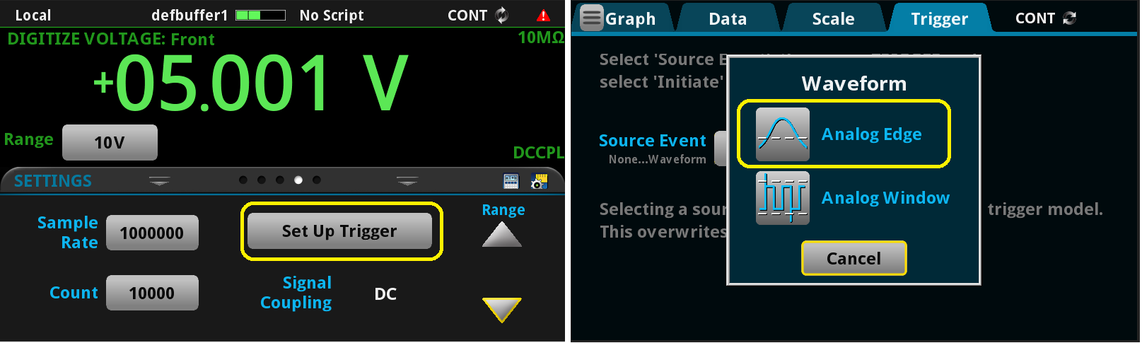
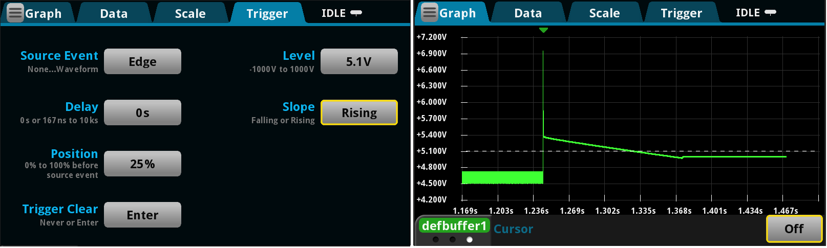
After setting up the 2230A power supply to output 10V at 3A on two output channels (to ensure enough current is made available for the power conversion), we set up the 2380 electronic load to sink constant current of 7A. The output of the 2230A is turned on, while the 2380 is left off. We configure the DMM6500 to digitize voltage, setting the sample rate to 1 MS/s for a count 10k readings then touch the Set Up Trigger button to reveal the waveform capture options. We choose Analog Edge from the Source Event options.
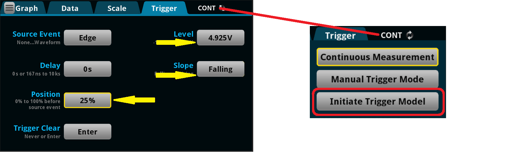
Since we expect some decline in voltage when we apply our load, we set the level to 4.925 V and the slope such that we are looking at the falling edge. If we so choose, we can use the Position option to adjust the horizontal presentation of the waveform on the graph. To arm the DMM6500 and start monitoring for the event, we touch the CONT annunciator in the upper left corner of the display, revealing a drop-down menu of triggering options, and choose Initiate Trigger Model.
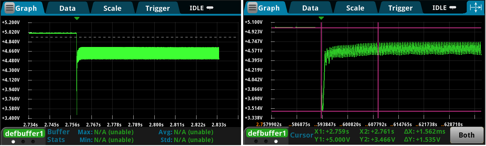
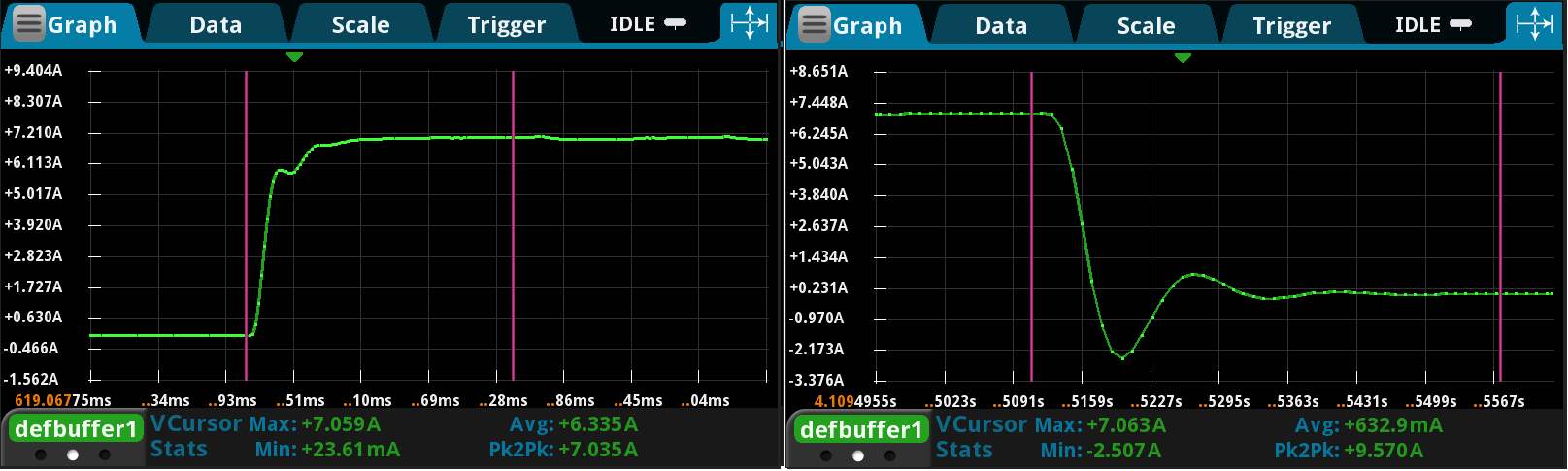
Finally, we turn on the 2380 electronic load, applying an effective step function that sinks 7A. The DMM6500 will perform the sampled waveform capture which is provided in the Graph tab. This shows the transient response for when a load is applied to the output of the LM25088MH switching supply. We can further evaluate by using the touch screen of the DMM6500 to zoom into the area of interest and turn on the cursors to get metrics on the changes in signal level (y-axis info) versus time (x-axis info). We can see that the switching supply stabilizes after about 1.5 milliseconds. Even more interesting is the large dip that the application of the load produced, driving the output voltage levels as low as 3.466 V.
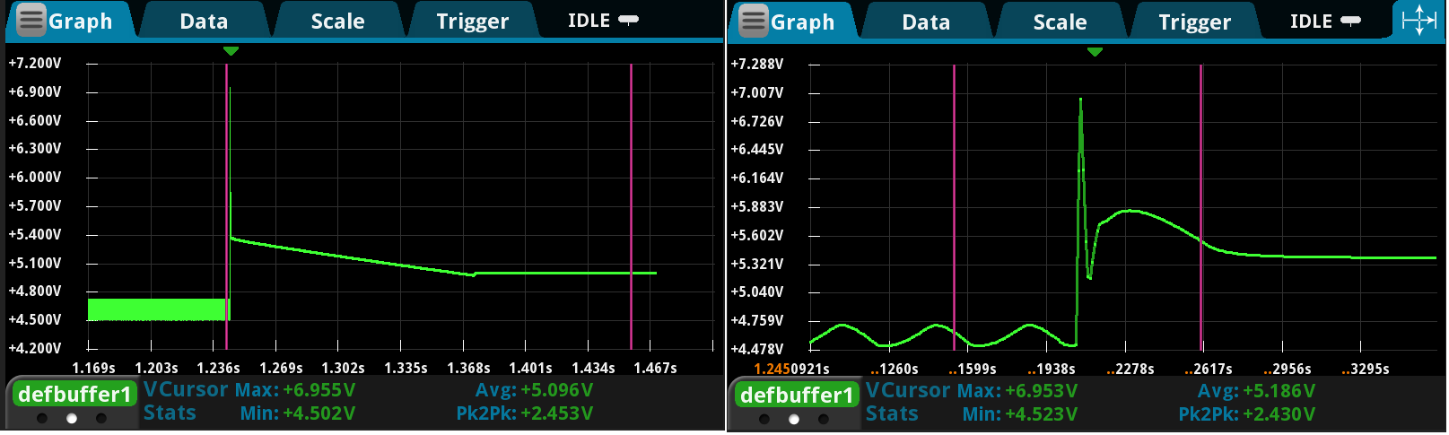
Just as important as the transient recovery when a load is applied is what happens when that same load is removed. To capture this, we touch the Trigger tab on the DMM6500, changing the level to 5.1 V and the slope to Rising. We can trigger the DMM the same as we did before (with the drop-down menu option) or now just press the TRIGGER key to the left of the DMM display on the front panel of the instrument. After doing so, we simply turn off the 2380 electronic load, and we can see the switching power supply recovery waveform on the graph of the DMM6500.
Instead of enabling both horizontal and vertical cursors on our display, we use just the latter and swipe on the information bar at the bottom of the screen to reveal the VCursor Stats. This will give us basic statistical information on the data points bounded between the vertical bars. Therefore, we do not need to enable and adjust the horizontal cursors to determine that the switching supply is peaking at 6.953 V when the load is removed. We can set the right-hand cursor to where the small dip occurs prior to the output becoming flat to find that the recovery response time is approximately 125 milliseconds. Alternatively, we could zoom in to the peak point area to get a better view of how the voltage signal is behaving.
Now let us turn our attention to the current signal with this same circuit, but connect the DMM6500 in series with the 2380 electronic load. Take note that because we are working with a substantial amount of current (7 A) we will need to use the 10 A current input connection available on the rear of the DMM:
We set up our triggering options similar to before, though this time we trigger at the halfway point of the anticipated 7 A signal and keep the slope set to Rising.
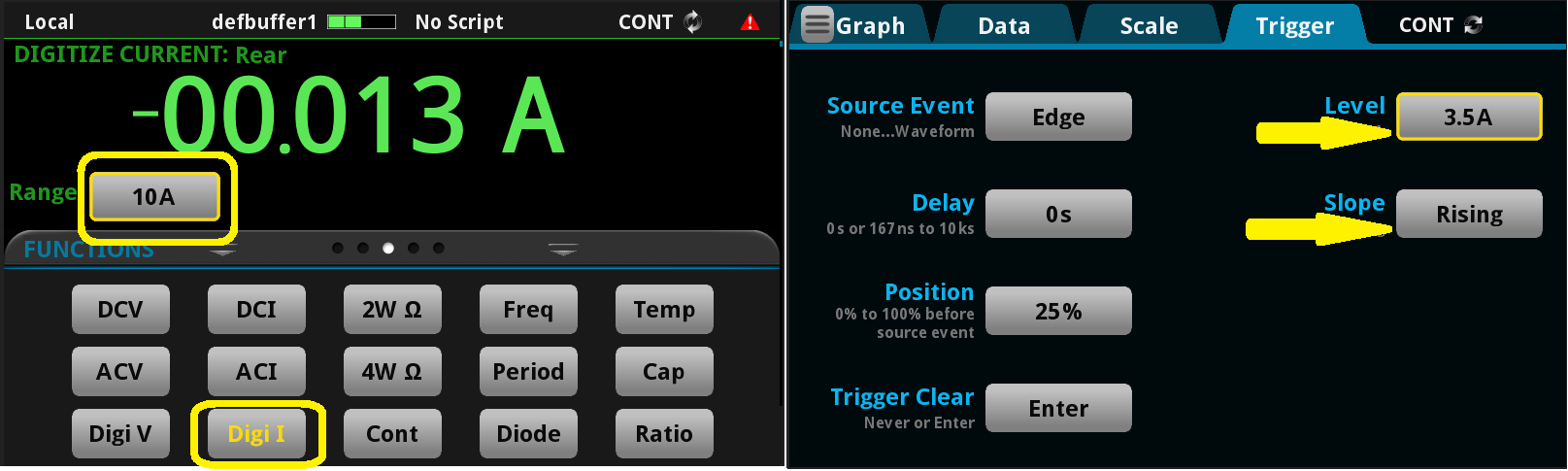
Again, we trigger the DMM6500 (via drop-down) and then turn on the 2380 electronic load – the DMM has no problem responding to the waveform event. We repeat this process for when the load is removed also using the on-screen cursors for quick data analysis, showing the current dipping to -2.5 A.
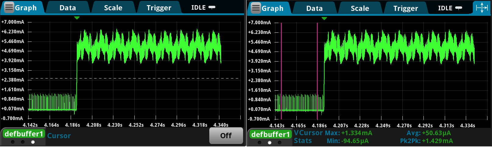
While our attention has been focused on high-power waveform capture, we should close by noting the current sensitivity advantage that a digital multimeter offers. Many devices being designed today must consume as little power as possible such that they conserve battery life. This same switching circuit from the LM25088MH evaluation unit may be integrated into a low-power wireless design where the low current levels drawn by the individual components must be evaluated as they are transitioned into different states (sleep, standby, sense, process, etc.). The process for capturing low current waveform events is the same as outlined above; however, the lower ranges let the user monitor minute current levels. For instance, if we set our load to 5 mA and use the 10 mA range on the DMM6500, we are able to visualize micro Amp readings.
I hope this blog post gives you insight into transient recovery measurements and a feel for a small part of the more than 500 products in the Keithley portfolio that are used to source, measure, connect, control or communicate direct current (DC) or pulsed electrical signals. To get the full story – and to keep your power supplies from dropping balls – go to: https://www.tek.com/keithley.