Свяжитесь с нами
Живой чат с представителями Tektronix. С 9:00 до 17:00 CET
Позвоните нам
С 9:00 до 17:00 CET
Загрузить
Загрузить руководства, технические описания, программное обеспечение и т. д.:
Обратная связь
Power Supply Measurement and Analysis with 4/5/6-PWR Application Software

Power Supply Measurement and Analysis with 4/5/6-PWR Application Software
From portable electronics to industrial and energy systems, designers must evaluate steady-state performance, and dynamic behaviors such as switching losses, control loop stability, and transient response. Oscilloscope-based tools enable engineers to achieve these goals with accurate, repeatable measurement techniques that can capture voltage, current, and power relationships across multiple domains of operation.
This application note describes:
- How to setup for accurate power measurements, including probe deskew, probe offset correction, and current probe degaussing.
- How to optimize the latest GaN and SiC designs and perform switching analysis on transistors.
- How to characterize inductors and transformers to determine power supply stability and efficiency, and characterize the frequency response of a power supply control loop.
- How to evaluate the output of a DC power supply and perform inverter ride-through analysis.
- Discusses differential and current probes, including IsoVu isolated probes.
The instruments used in this application note are Tektronix 4, 5, and 6 Series B Mixed Signal Oscilloscopes equipped with Advanced Power Measurement and Analysis software (Options 4-PWR, 5-PWR, or 6-PWR). These platforms, when combined with appropriate voltage and current probes, provide a scalable and consistent measurement environment for a wide range of power electronics applications.
Introduction
Today’s power supply designers are faced with increasing pressure to achieve power conversion efficiencies of 90% and even higher. This trend is driven by demand for longer battery life in portable electronics, the Internet of things and demand for “greener” products that consume less power. Many designs are replacing silicon FETs and IGBTs with GaN or SiC switching devices. As always, the pressure of time to market continues to push faster (but still accurate) testing.
The 4, 5 and 6 Series MSOs with their FlexChannel® inputs and innovative graphical user interfaces enables designers to test multiple test points at one go, thereby speeding up testing. The Advanced Power Measurement and Analysis option (4-PWR, 5-PWR and 6-PWR) automates the setup process for key power measurements and provides tools to evaluate test results based on norms and standards in power supply design.
This application note gives an overview of how to make important power supply measurements using a Tektronix 4, 5 or 6 Series MSO oscilloscope with 4-PWR, 5-PWR, or 6-PWR power analysis software.
Preparing for Power Supply Measurements
In order to make accurate measurements, the power measurement system must be setup correctly to precisely capture waveforms for analysis and troubleshooting. Important topics to consider are:
- Eliminating skew between voltage and current probes
- Eliminating probe offset
- Degaussing your current probe
ELIMINATING SKEW BETWEEN VOLTAGE AND CURRENT PROBES
To make power measurements with an oscilloscope, it is necessary to measure voltage across and current through the device under test. This task requires two separate probes: a voltage probe (often a high voltage differential probe) and a current probe. Each voltage and current probe has its own characteristic propagation delay and the edges produced in these waveforms will probably not be aligned. The difference in the delays between the current probe and the voltage probe, known as skew, causes inaccurate amplitude and timing measurements.
Since skew creates a timing delay, it can cause inaccurate measurements of timing differences, phase, and power factor. Many measurement systems can “auto-calibrate” for delays internal to the instrument, but when you add probes to your system you must compensate for differences in probe amplifiers and cable lengths.
The 4, 5 or 6 Series MSOs allow you to compensate for the delays from your probe tips to the measurement system to ensure you make the most accurate timing measurements. You can manually deskew the probes by connecting your probes to the same waveform source, and adding delay to the signal path of the faster signal. This allows the signals to be aligned in time without having to physically add cable length to the shorter probe cable.
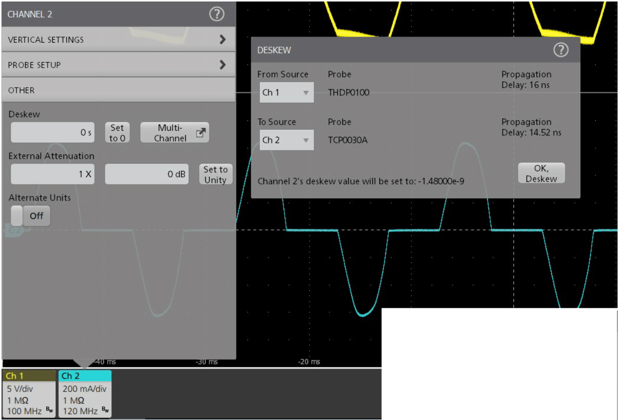
Figure 1. Static skew compensation between a differential voltage probe and current probe BEFORE Adjustment. These probes have onboard memory that stores their nominal propagation delays.
The 4, 5 and 6 Series MSOs also provide a one-button "static" deskew feature. Figure 1 shows an example of skew between two TekVPI® power probes. The oscilloscope reads the nominal propagation delays from the probes and calculates that there is a difference of about 1.48 ns of delay between the two probes. Simply pressing the OK, Deskew button adjusts the relative timing between the signals.
Figure 2 shows the same test setup used in Figure 1 after the static deskew function has been run. If non-Tektronix probes are used, you will need to manually deskew the voltage and current waveforms, and configure the current probe settings.
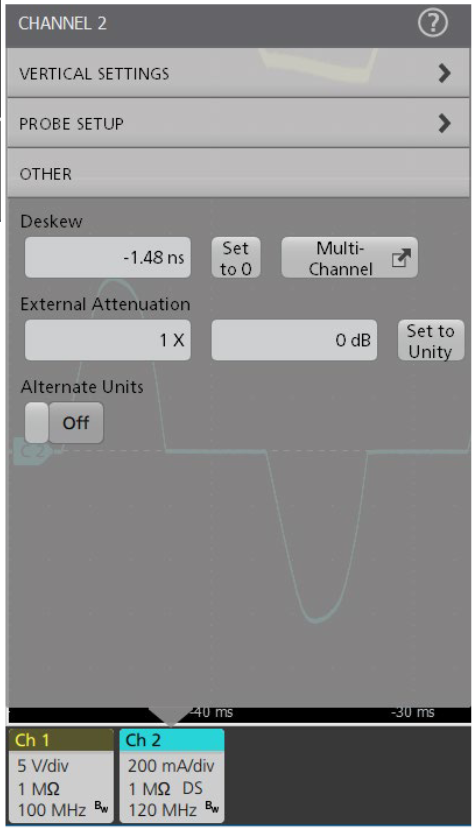
Figure 2 shows the same test setup used in Figure 1 after the static deskew function has been run. If non-Tektronix probes are used, you will need to manually deskew the voltage and current waveforms, and configure the current probe settings.
ELIMINATING PROBE OFFSETS
Differential probes may have a slight voltage offset. This offset can affect accuracy and should be removed before proceeding with measurements. Most differential voltage probes have built-in DC offset adjustment controls, which makes offset removal a relatively simple procedure.
Similarly, it may be necessary to adjust offset on current probes before making measurements. Current probe offset adjustments are made by nulling the DC current to a mean value of 0 amperes or as close as possible. TekVPI probes, such as the TCP0030A AC/DC current probe, have an automatic Degauss/AutoZero procedure built in that’s as simple as pressing a button on the probe compensation box, as shown in Figure 3.
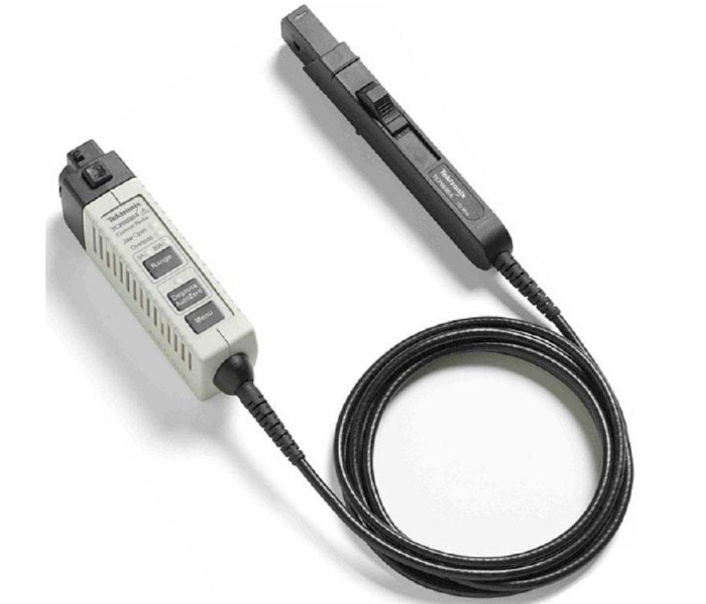
Figure 3. Tektronix TCP0030A AC/DC Current Probe with Degauss/AutoZero.
DEGAUSSING YOUR CURRENT PROBE
Degaussing removes any residual DC flux in the core of the transformer, which may be caused by a large amount of input current. This residual flux results in an offset error that should be removed to increase the accuracy of the measurements being made.
Tektronix TekVPI current probes offer a degauss warning indicator that alerts the user to perform a degauss operation. A degauss warning indicator is important since current probes may have significant drift over time, which can significantly affect measurements.
Addressing wide bandgap testing challenges
Until recently, switching measurements on the high side of half-bridge switching stages were almost impossible. Any measurement relative to the switching node, including high-side VDS and voltages across current shunts, suffered from distortion due to the significant common mode voltage signal impinging on the differential signal. This problem is worse with wide bandgap devices, such as GaN and SiC transistors, as switching frequencies increase and the need to optimize brand new designs becomes imperative. The unmatched common mode rejection of IsoVu probes and the automation of Advanced Power Measurement and Analysis make an unbeatable combination for optimizing the latest GaN and SiC designs.
Figure 4. Many power supply topologies require measurements of small differential voltages in the presence of high common mode signals. For example, VGS on the high side of a half-bridge switching stage often move up and down 100s of volts relative to ground. IsoVu™ Isolated Measurement Systems offer extremely high common mode rejection
Input Analysis
Line measurements characterize the design’s reaction to changing inputs, the design’s current and power draw, and the design’s distortion of the line current. Some measurements, such as power consumption, are critical specifications. Others, such as power factor and harmonics, may be limited by regulations.
POWER QUALITY MEASUREMENTS
In 4-PWR, 5-PWR and 6-PWR, Power Quality measurements are a set of standard power measurements. They are often performed on AC line inputs, but can also be applied to AC outputs of devices such as power inverters. These measurements include:
- Frequency
- RMS voltage and current
- Crest Factor (voltage and current)
- True, reactive, and apparent power
- Power factor and phase
Making the measurement
Power quality measurements are easily made by using a differential probe to measure the line voltage of the system and a current probe to measure the line current of the system. This same setup may be used to measure current harmonics as well.
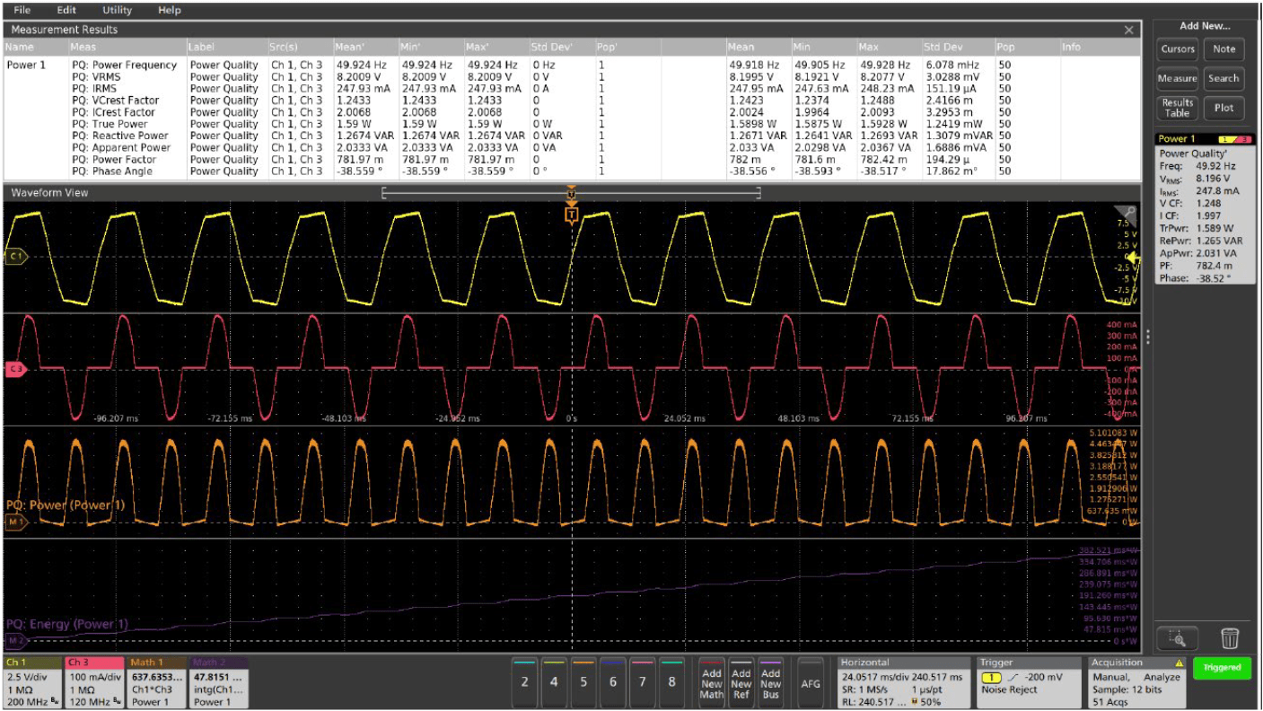
Figure 5. Power quality measurements paint a rich picture of the AC line. Line voltage is the upper waveform. Current is the red waveform. Instantaneous power is the orange waveform. The results badge (upper right) shows a summary of the line characteristics, and the results table in the upper section can be activated for more detailed data and statistics.
Measurement results
- Frequency: The frequency in Hertz of the voltage waveform
- VRMS: The Root-Mean-Square value of the displayed voltage waveform
- IRMS: The Root-Mean-Square value of the displayed current waveform
- V Crest Factor: The peak amplitude of the voltage divided by the RMS value of the voltage
- I Crest Factor: The peak amplitude of the current divided by the RMS value of the current
- True Power: The real power of the system measured in Watts (W)
- Reactive Power: The imaginary power temporarily stored in inductive or capacitive elements, measured in Volt-Amperes-Reactive (VAR)
- Apparent Power: The absolute value of the complex power measured in Volt-Amperes (VA)
- Power Factor: Ratio of the True Power to the Apparent Power
- Phase: The angle between the True and Apparent Power vectors, in degrees
HARMONICS
Current harmonics occur when non-linear devices distort the flow of current into the circuit. Linear circuits draw current only at the fundamental line frequency, but non-linear circuits draw current at multiples of the fundamental frequency, with a different amplitude and phase for each harmonic.
When currents with harmonics flow through the impedance of the electrical distribution system, voltage distortion can result. Heat can build-up in cabling and transformers. And as the number of switching supplies connected to the grid increases, the harmonic distortion on the grid also increases.
Thus, standards have been designed to limit the impact on power quality from non-linear loads. Standards such as IEC61000- 3-2, MIL-STD-1399 and DO-160G have been developed to limit harmonics.
The IEC61000-3-2 standard limits the current harmonics injected into the public mains power supply system. It applies to all electrical and electronic equipment that has input current up to 16A per phase that will be connected to public low voltage distribution systems (230V AC or 415V AC 3 phase). The standard is further divided into Class A (balanced 3-phase equipment), Class B (portable tools), Class C (lighting equipment and dimming devices) and Class D (equipment with unique current waveform requirements).
MIL-STD-1399 lays out specifications and testing requirements for equipment (loads) to maintain compatibility with shipboard AC power systems, from computers and communications equipment to air conditioners. DO-160G standards are for airborne systems.
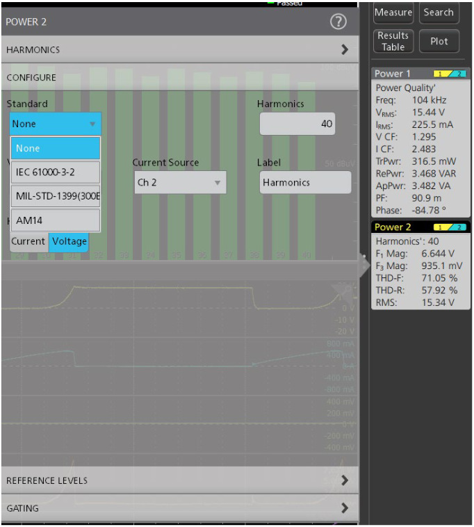
Figure 6. Setting up a basic current harmonics analysis requires just a few settings. This example shows settings for a pre-compliance check against industry standards.
The power analysis applications make it easy to measure current harmonics. It can display the measurement results in both tabular and graphical formats. It also enables designers to quickly compare performance of their devices against compliance standards before going through certification -- an often time-consuming and expensive process. Having these measurement capabilities available in the oscilloscope, not only speeds up debugging, but can help avoid last minute design changes to meet regulatory requirements.
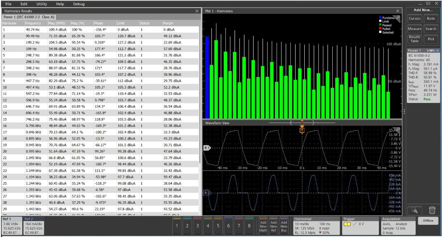
Figure 7. Harmonics results. The non-sinusoidal current waveform with can be seen in the lower right. The harmonics bar chart shows harmonic content on a decibel scale. The odd harmonics are most significant, but well within the IEC 61000-3-2 limits.
Making the measurement
Use a differential voltage probe to measure the line voltage. Use a current probe to measure the line current.
If you want to compare the harmonics in your design against limits in the IEC 61000-3-2 standard, line frequency must be defined, and the class type needs to be selected. In the case of Class C or D standards, the input power, power factor and fundamental current will also need to be entered. The analysis package will load a pre-defined limit table and make comparisons between measured harmonics and limits. The pre-compliance results will be presented as shown in Figure 8.
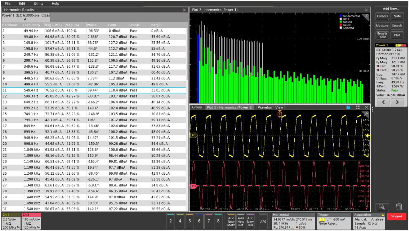
Figure 8. Up to 100 Harmonics may be displayed in graphical form. The table shows IEC 61000-3-2 pre-compliance testing results. Based on your settings the analysis package will load a pre-defined limit table and make comparisons between each measured harmonic and limits.
Measurement results
- The Results badge shows the Harmonics standard selected, Fundamental Harmonic and 3rd Harmonic magnitude, THD-F, THD-R, RMS value and Pass/Fail status.
- Individual harmonics can be selected and measurement values are linked between the results badge, bar graph, and results table.
- Harmonics Results Table includes:
- Current harmonics may be shown in units of decibel microamperes (dBµA) or amperes (A)
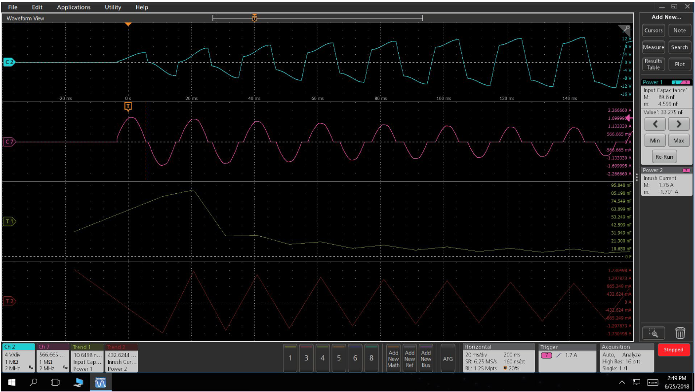
Figure 9. Automated inrush current measurement and capacitance measurement being performed on the current on Channel 7.
INRUSH CURRENT AND INPUT CAPACITANCE
In general, inrush current occurs when a power supply is first turned on. The power converter draws a relatively high current as its input capacitance charges up. After the initial inrush, the current settles to a steady state unless other system changes occur. Inrush current measurements can provide important information non the design of a power supply, including sizing protection devices. In extreme cases, inrush current can cause voltage sags on the AC line.
The power analysis software provides an automated inrush measurement. It identifies inrush regions and annotates them on the display. It then calculates the inrush current within that region.
Inrush current and input capacitance are directly related, and both provide important insights into the startup characteristics of a power converter.
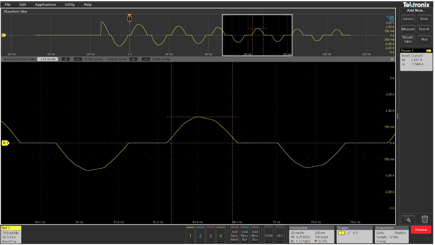
Figure 10. Inrush occurs during a power supply turn-on. The current waveform shows gradually reducing peaks before it reaches steady state.
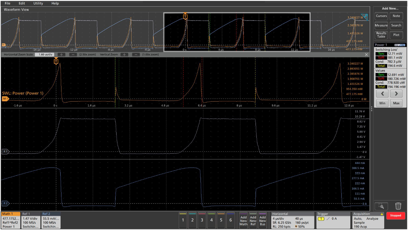
Figure 11. Switching Loss Measurements. The upper trace (orange) is calculated by multiplying current and voltage for instantaneous power. Loss measurements are performed on the instantaneous power waveform. Each loss region is annotated with colored markers that correspond to measurement labels. The bottom waveforms are the voltage across the switch and current through the switch.
Switching Analysis
Measurements in the switching stages of the power supply confirm that the converter is functioning correctly, quantify sources of loss, and confirm that devices are operating within normal ranges.
SWITCHING LOSS MEASUREMENTS
Turn-on losses occur as various physical and parasitic capacitors are charged, inductors generate magnetic fields, and related transient resistive losses occur. Likewise, when the switching supply turns off there is energy still available to discharge and interact with various components even though the main power has been removed, and so losses occur here too.
Making the measurement
To make a switching loss measurement, the oscilloscope must measure voltage across the switching device and current through the device. The switching loss results are presented as shown in Figure 11.
Measurement results
- Ton: The mean of the Turn On power and energy loss values for each cycle
- Toff: The mean of the Turn On power and energy loss values for each cycle
- Total: The mean of the Total Average Power Loss and Average Energy values for each cycle
- Left and right arrow buttons let you traverse through the switching cycles and zero-in on problem areas
- Measurements can also be viewed in a Results Table. The table shows accumulated measurement results for all switching cycles for quick review.
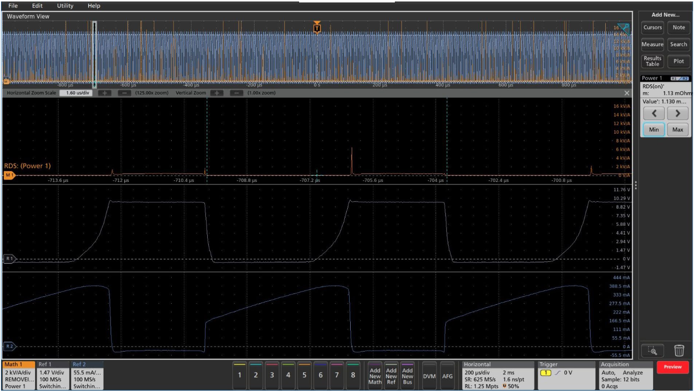
Figure 12. RDS(on) measurement. The Ch1 (yellow) waveform is the FET VDS voltage and the Ch2 (cyan) waveform is the FET current. The waveforms are inverted in phase to correctly indicate that the current is high in the conduction region. The Math plots the RDSon value and the results badge shows the minimum RDSon value calculated as per the Math waveform.In this case it is 1.13 mOhms.
RDS (ON)
This measurement characterizes the drain-to-source resistance of the switching device during the conduction portion of the switching cycle, when the device is ON and conducting current. The dynamic on-resistance is ratio of the voltage across the device when it is turned ON to the current flowing through the device. Using cursor gating capability you can accurately measure RDS(on), an important contributor to losses in the switching device.
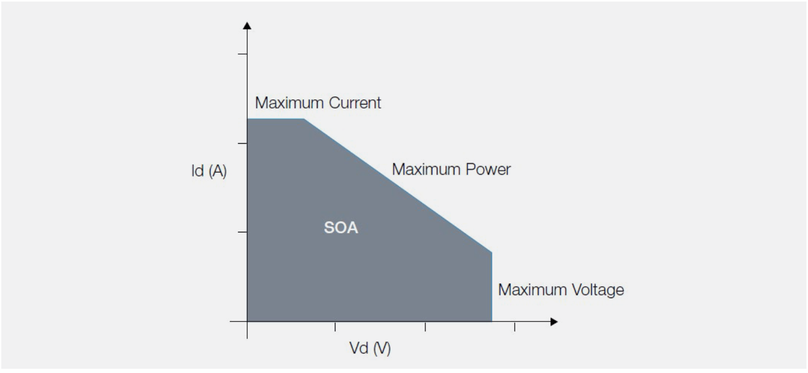
Figure 13. Safe Operating Area (SOA) graph of a transistor.
SAFE OPERATING AREA
The safe operating area (SOA) of a switching transistor defines the current that can safely run through the transistor at a given voltage. The SOA is usually defined in the datasheet of BJT, MOSFET, or IGBT switching transistors. It is given as a plot of VCE (or VDS for a FET) versus ICE (or IDS), and describes the ranges over which the transistor can operate without degradation or damage.
Power analysis software lets you transfer the SOA from the device datasheet into the 4, 5 or 6 Series MSO. Then you can measure voltage and current on the actual, in-circuit device as you vary the operating conditions of your power supply design. The oscilloscope records the V-I plots and can indicate whether any parameters go outside the SOA.
Making the measurement
One of the main challenges with determining the SOA of a transistor while operating in a power supply is accurately capturing voltage and current data under a variety of load scenarios, temperature changes and variations in line input voltages. The analysis package simplifies this task by automating data capture and analysis. The measurement setup requires probing the voltage across and the current through the switching transistor.
The next step is to set up the SOA mask. As shown in Figure 15, the SOA Mask editor lets you enter the SOA limits for the transistor, as defined in its datasheet or by your own standards.
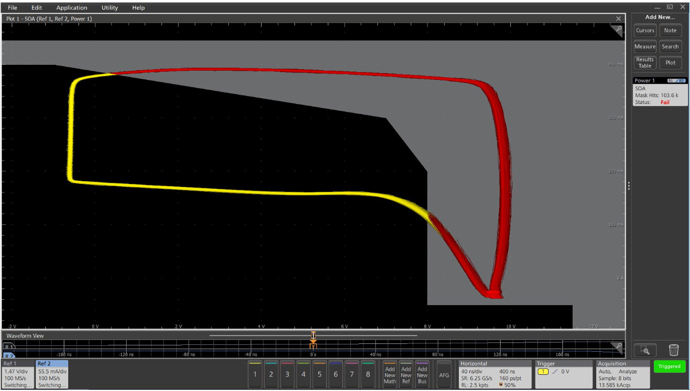
Figure 14. SOA using 5-PWR. If the data points fall inside the mask zone, they are yellow to indicate ‘pass’ and if they fall outside the mask zone, they are red to indicate ‘fail’. In this example, the V-I curve has gone outside the SOA, subjecting the switching device to excessive stress.
Measurement results
After completing the setup, the SOA test results are presented as shown in Figure 14. The voltage and current waveforms are plotted in a single record in XY mode. The plot shows all the data for a single acquisition cycle.
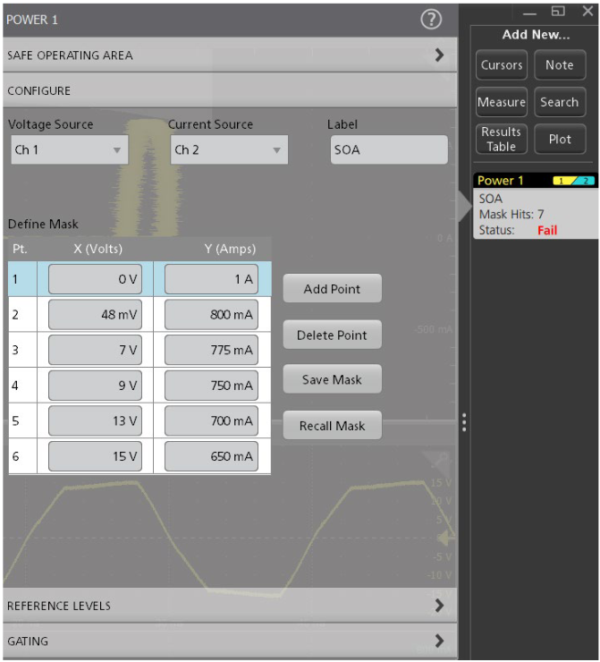
Figure 15. SOA Mask Editor window. The mask is defined by a set of (voltage, current) coordinates taken from the switching device datasheet, or may be user-defined
The results badge shows the number times the device went outside the SOA mask and gives a pass/fail verdict.
Magnetic Analysis
Inductors and transformers are used as energy storage devices in both switch-mode as well as linear power supplies. Some power supplies also use inductors in filters at their output. Given their important role in power converters, it is essential to characterize these magnetic components to determine the power supply’s stability and overall efficiency.
Magnetics analysis in 4/5/6-PWR automates the following groups of measurements: inductance, magnetic loss, and B-H parameters.
INDUCTANCE
Inductors exhibit increasing impedance with frequency, impeding higher frequencies more than lower frequencies. This behavior is known as inductance and is measured in units of Henries. The inductance of devices can be measured automatically with an oscilloscope equipped with power analysis software.
Making the measurement
The 4/5/6-PWR applications integrate the voltage over time and divides by the change in current to calculate the inductance value. Measurements are made by probing the voltage across and the current through the magnetic component. The inductance measurement results are presented along with several other measurements in Figure 15. The yellow (Ch1) waveform is the voltage across the inductor and the cyan waveform (Ch2) is the current through the inductor. Note that the B-H curve is also displayed.
Measurement results
Inductance: The inductance value of the device or circuit
MAGNETIC LOSS
An analysis of magnetic power losses is an essential part of a comprehensive loss analysis of a switching supply. The two primary magnetic losses are core losses and copper losses. The resistance of the copper winding wire contributes to the copper losses in a power supply. Core losses are a function of eddy current losses and hysteresis losses in the magnetic core. Core losses are independent of DC flux, but are influenced by the AC flux swing and the frequency of operation.
Making the measurement
4/5/6-PWR are capable of calculating the magnetic loss in a single winding inductor, a multiple winding inductor, or even a transformer.
In the case of a single-winding transformer, a differential probe is connected to measure the voltage across the primary winding. A current probe measures the current through the transformer. The oscilloscope and power measurement software can then automatically calculate the magnetic power loss.
The magnetic power loss results are presented as shown in Figure 16.
Measurement results
Power Loss: The total power loss due to the magnetic component
MAGNETIC PROPERTIES (B-H CURVE)
Magnetic flux density B, measured in units of Tesla, is the strength of the magnetic field. It determines the force that is exerted upon a moving charge by the magnetic field. The magnetic field intensity or field strength H, measured in A/m, is referred to as the magnetizing force. The magnetic permeability of a material, µ, is measured in H/m. It measures the degree of magnetization of the material due to the applied magnetic field.
Physical characteristics such as the magnetic length and the number of windings around the core help determine the B and H of the magnetic material. B-H curve plots are often used to verify the saturation (or lack thereof) of the magnetic elements in a switching supply and provide a measure of the energy lost per cycle in a unit volume of core material. The curve plots the magnetic flux density, B, against the field strength, H. Since both B and H depend on the physical characteristics of the magnetic component, such as the magnetic length and the number of windings around the core, these curves define the performance envelope of the component’s core material.
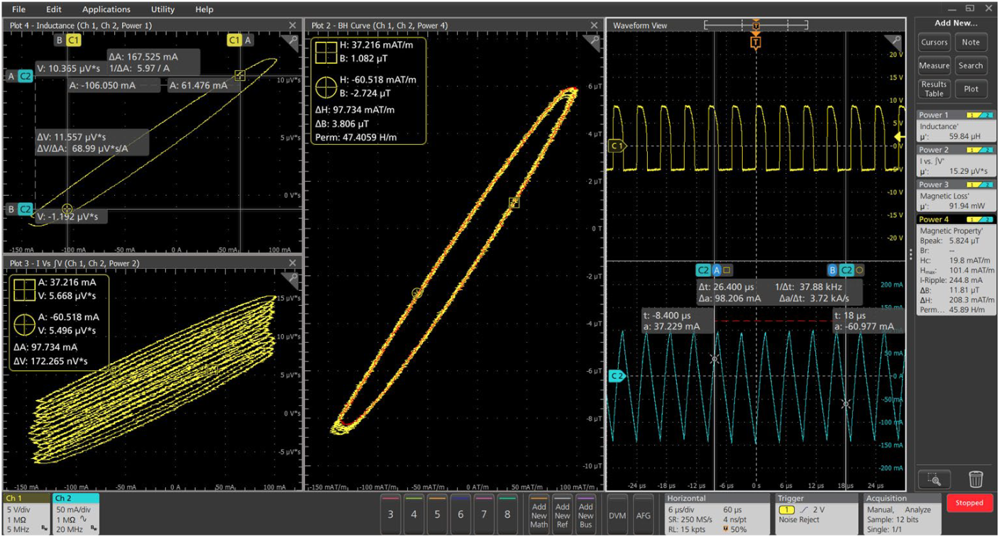
Figure 16. Magnetic measurements on an inductor. The Ch1 (yellow) waveform is the voltage across the inductor and the Ch2 (cyan) waveform is the inductor current. The B-H curve is shown in the center of the display. Inductance, magnetic loss, and magnetic properties are shown in results badges on the right.
Making the measurement
In order to generate a B-H plot, the voltage across the magnetic element and the current flowing through it are measured. In the case of a transformer, the currents through the primary as well as secondary windings are of interest. The number of turns of the inductor (N), the magnetic length (l) and the cross-sectional area of the core (Ae) must first be entered in the configuration panel, before the power analysis software can compute a B-H curve plot.
A high-voltage differential probe is connected to channel 1 on the oscilloscope and across the primary winding of the transformer. This measured voltage is a result of the magnetic induction B of the magnetic component. Channel 2 measures the current through the primary with a current probe. Current probes are also used to measure the current through the secondary windings on channel 3 and channel 4, if needed. The power analysis software can then calculate the magnetizing current using the data from oscilloscope channels 2, 3 and 4. The magnetizing current value is then used to determine the H component.
The magnetic property results are presented as shown in Figure 16.
Measurement results
- ΔB: The change in flux density
- ΔH: The change in field strength
- Permeability: The degree of magnetization of the material
- Bpeak: The maximum magnetic flux density induced in a magnetic component
- Br: The point on the curve where H = 0 but B still has a positive value. This is known as the Remanence of the component, a measure of its Retentivity. The higher the remanence, the more magnetization the material will retain.
- Hc: The point on the curve where B = 0 and H is a negative value. This represents the external field required to cause B to reach zero. This value of H is known as the coercive force. A small coercive force value means that the component can be demagnetized easily.
- Hmax: The maximum value of H at the intersection of the H-axis and the hysteresis loop
- I-ripple: The peak-to-peak value of the current
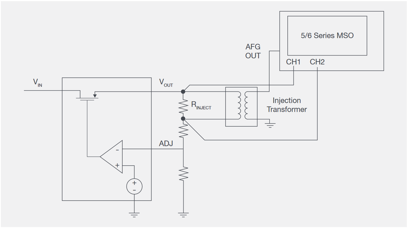
Figure 17. An isolation transformer / injection transformer is used to isolate the grounded signal source from the floating injection resistor.
Frequency Response Analysis
CONTROL LOOP RESPONSE
Control loop response analysis (often called Bode plots, after the resulting curves) helps to characterize the frequency response of a power supply control loop. The Bode plot represents the gain and phase shift of the feedback loop computed over a range of frequency values, providing valuable information about the speed of the control loop and stability of the power supply. It may be measured with a vector network analyzer (VNA) but can also be measured with an oscilloscope and function generator.
To measure the response of a power system a known signal must be injected into the feedback loop. For this measurement the Arbitrary/Function Generator (AFG) option in the 4/5/6 Series is used to generate sinewaves over a specified range of frequencies. The DC-DC converter or LDO must be configured with a small (5-10Ω) injection resistor / termination resistor in its feedback loop so that a disturbance signal from the function generator may be injected into the loop.
An injection transformer with a flat response over a wide bandwidth is connected across the injection resistor and isolates the grounded signal source from the power supply. The Picotest J2101A Injection Transformer has a range of 10Hz-45MHz which aligns well with the function generator option for the 4/5/6 Series MSO. Low capacitance, low attenuation passive probes such as the TPP0502 are recommended for the voltage measurements. This enables measurements with vertical sensitivity of 500 µV/div on the 6 Series MSO, and 1 mV/div on the 4/5 Series MSO.
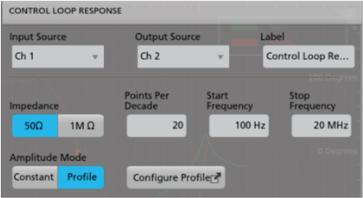
Figure 18.The start and stop frequency, amplitude, and points-per-decade determine the stimulus the generator will inject into the control loop.
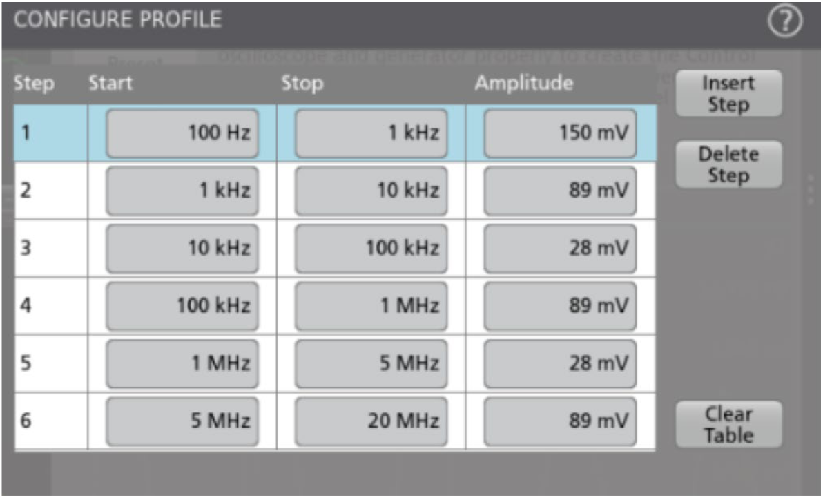
Figure 19. An amplitude profile may be used to improve signal-to-noise ratio (SNR) of measurements. It enables application of lower amplitudes at frequencies where the DUT is sensitive to disturbances and higher amplitudes at frequencies where it is less sensitive.
After making connections, the stimulus sweep must be configured. The 4/5/6-PWR software supports constant amplitude and profile amplitude methods. The constant amplitude sweep maintains the same amplitude at all frequencies. The profile method allows you to specify different amplitudes at frequency bands you define. The amplitude profile method may be used to improve the signal-to-noise ratio (SNR) of the measurements.
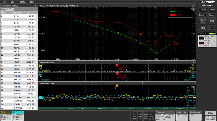
Figure 20. The software computes gain (green trace) as 20log (Vout/Vin). The red trace represents the phase shift between the injected signal and the output relative to -180°. Phase margin (PM) is measured where the gain curve crosses zero dB. Gain margin (GM) is measured when the phase curve crosses the zero-degree mark. The table shows gain and phase at each frequency.
Phase margin is measured at the gain crossover frequency, which occurs at the frequency where the gain plot crosses 0 db. The corresponding point on the phase plot gives the phase margin.
Gain margin is measured at the phase crossover frequency, which occurs when phase crosses through -180 degrees. Since phase is plotted relative to -180, this shows up as a 0 crossing. The corresponding gain value at this phase crossover frequency gives the gain margin.
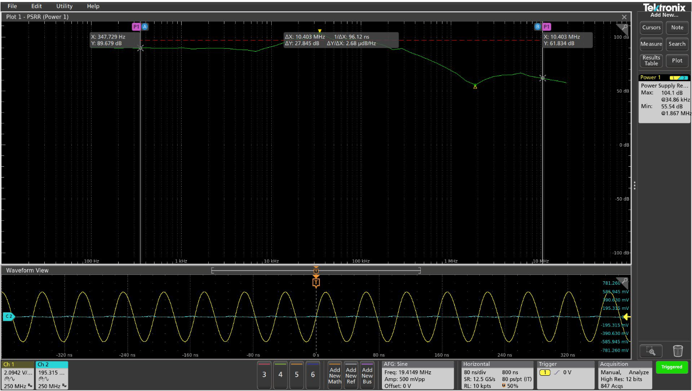
Figure 21. The PSRR plot shows the attenuation of AC applied to the input of the supply on the output of the supply.
POWER SUPPLY REJECTION RATIO (PSRR)
Power supply rejection ratio characterizes a power supply’s ability to prevent AC noise on its input from appearing on its DC output. To perform a PSRR test, a swept sinusoidal stimulus is applied to the input of the power supply. A DC + AC network summing device, such as Picotest’s J2120A line injector, is required for this measurement.
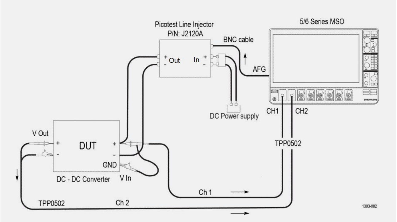
Figure 22. A line injector is used to add an AC stimulus from the function generator to the DC input of the power supply.
The 5/6-PWR software automates the sweep and takes measurements of the input output signals at each frequency. It computes the attenuation ratio as 20Log(Vin/Vout) at each frequency within the frequency band and plots the measurements on the display.
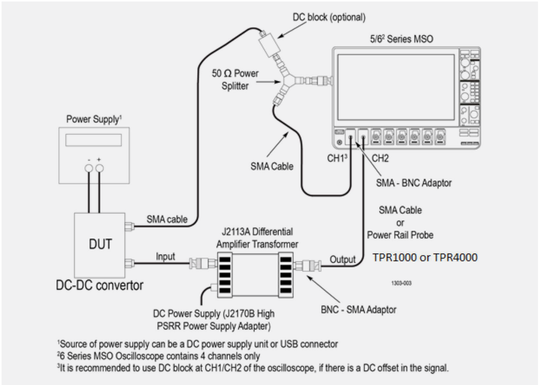
Figure 23. Impedance measurement setup. Power rail probes offer high sensitivity and high impedance at DC and 50 Ω AC input impedance for low loading. Alternatively, a P6150 probe may be used if available, or an SMA cable with DC block.
IMPEDANCE MEASUREMENTS
Characterizing the impedance of a power distribution network helps determine the impact of noise within the system. The impedance curve represents the impedance values across a specific frequency band. The DUT can be the combined impedance of PDN including board traces and capacitors, or a component or subsystem such as a Voltage Regulator Module (VRM).
Impedance measurements are often performed using VNAs, however the typical VNA cannot measure at low frequencies or measure low impedance values < 10 mΩ. The oscilloscopebased system can measure down to a frequency as low as 1 Hz. The scope-based solution also provides a display of both input and output signals from the DUT during the sweep, so time domain changes can be observed.
The oscilloscope also has the benefit of showing time domain waveforms, including the stimulus signal and the response, as the analysis is being performed. This is not possible with a VNA.
To perform the measurement, the grounded scope must be isolated from the DUT. A Picotest J2113A differential amplifier transformer serves this purpose in the example system shown in Figure 23. A 50 Ω power splitter is used to send the signal from the function generator to the DUT and Channel 1 on the oscilloscope.
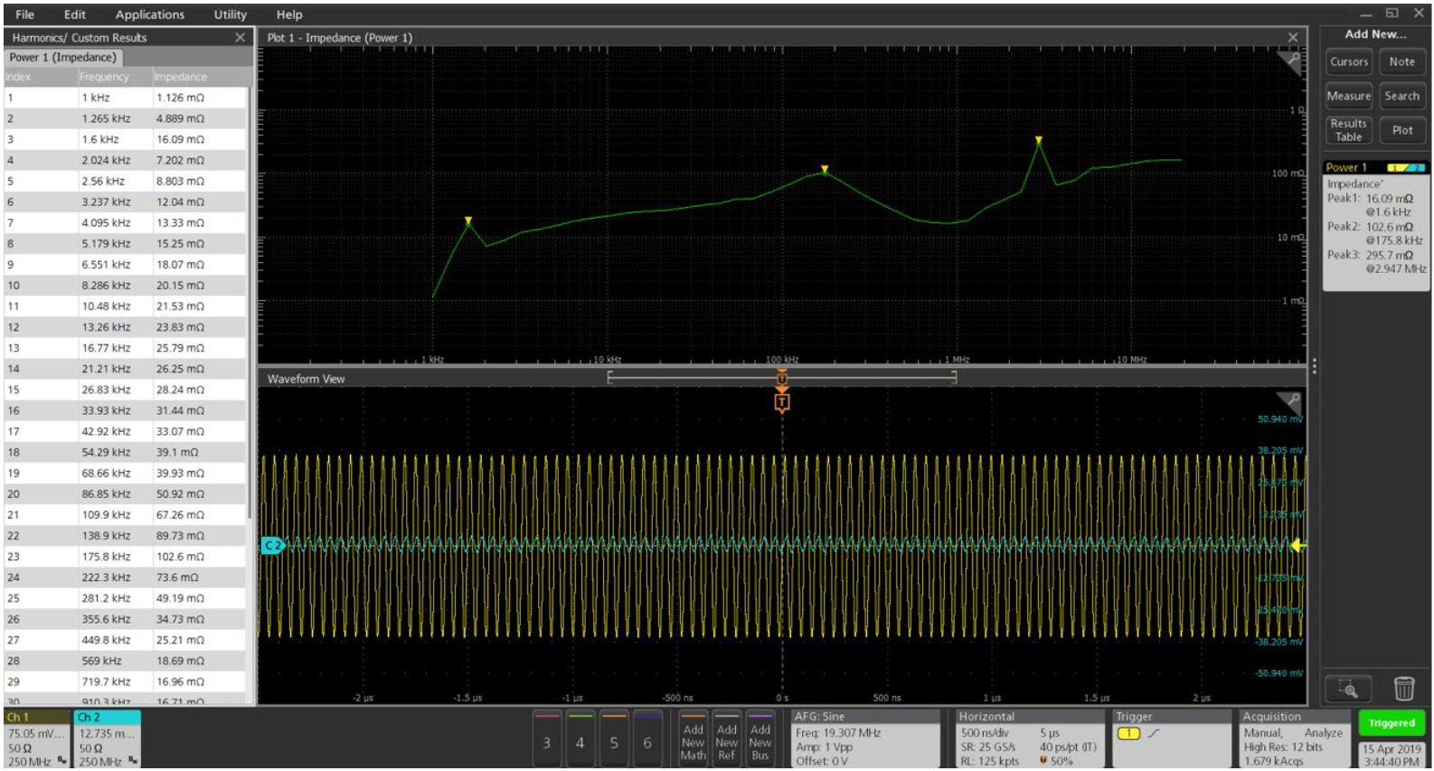
Figure 24. An impedance versus frequency measurement plot. The curve has three peaks indicating changes in impedance values as frequency is varied. The goal is a flat impedance plot, with any peaks falling below the target impedance. Cursors may be used to measure any point on the curve.
Output Analysis
The output of any DC power supply must be evaluated for regulation and noise. 4/5/6-PWR Advanced Power Measurement and Analysis software includes tools for quantifying and classifying ripple.
Line and Switching Ripple
Simply stated, ripple is the AC voltage that is superimposed onto the DC output of a power supply. It is expressed as a percentage of the normal output voltage or as peak-to-peak volts.
There are two kinds of ripple that show up at the output of a power supply. Line ripple measures the amount of ripple related to the line frequency. Switching ripple measures the amount of ripple detected from the switching supply output based on the switching frequency that you identify.
The output line ripple is usually twice the line frequency; whereas the switching ripple is typically coupled with noise and in the kHz frequency range. Separating line ripple from switching ripple is one of the biggest challenges in power supply characterization. Power analysis software greatly simplifies this task.
Making the measurement
To measure the ripple of the system, only a voltage probe is needed. The differential probe must be connected to the output of the system to measure the output line and switching ripple voltages.
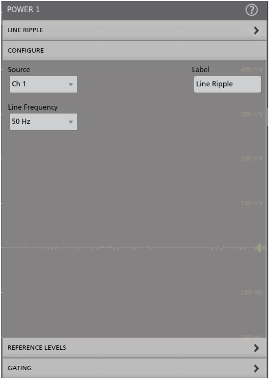
Figure 25. Line Ripple configuration tab for 5-PWR.
The configuration tabs (see Figure 25) for line and switching ripple are very similar. Both ripple measurements require the selection of input coupling (AC or DC) mode, bandwidth limit required (20MHz, 150/250MHz or Full) and the oscilloscope’s acquisition mode – Sample, Peak Detect or High Resolution (High Res). In the case of a line ripple measurement, the line frequency of the system, 50 Hz or 60 Hz or 400 Hz, must be defined. Switching ripple measurements require specification of the switching frequency.
Once the measurement has been configured, the results are presented as shown in Figure 26.
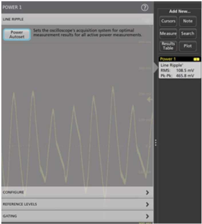
Figure 26. Switching Ripple results.
Measurement Results
Peak to Peak and RMS Ripple values: These are the peak to peak and RMS voltage values of the Line or Switching ripple of the system.
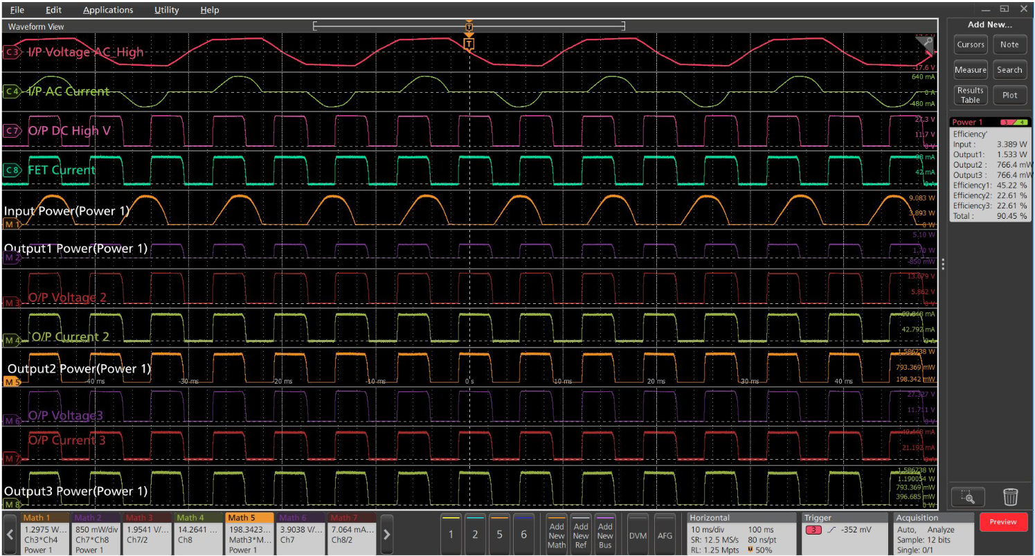
Figure 27. Efficiency measurement in which a single AC voltage and current are used to determine input power, and power is measured on three outputs simultaneously to find total efficiency.
Efficiency
High efficiency of devices or products is a critical differentiator in today’s competitive environment. Advanced Power Measurements and Analysis software enables you to easily measure the efficiency of your power conversion (AC-DC, AC-AC, DC-DC, DC-AC) products. For power products with up to 3 outputs, the Advanced Power Measurements and Analysis software enables designers to test the efficiency of the whole system at once, for faster testing and validation times.
Figure 27 shows the results of an efficiency measurement on an AC-AC converter with 1 input and 3 outputs, using a demo board and math signals to simulate a multi-output device. Each input and output voltage and current are measured (or simulated, in this case):
- Ch 3: Input Voltage
- Ch 4: Input Current
- Ch 7: Output 1 Voltage
- Ch 8: Output 1 Current
- Math 3: Output 2 Voltage
- Math 4: Output 2 Current
- Math 6: Output 3 Voltage
- Math 7: Output 3 Current
Note the use of custom labels in the above example, which enables easy identification. The application software automatically creates math power waveforms as needed. In the above example, these waveforms were created automatically:
- Math 1: Input 1 Power
- Math 2: Output 1 Power
- Math 5: Output 2 Power
- Math 8: Output 3 Power
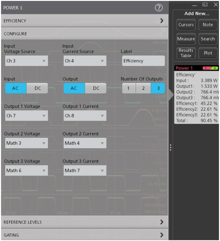
Figure 28. Efficiency measurement configuration allows user to configure the type of signal and up to 3 outputs.
The application calculates individual efficiencies and total efficiency of the device under test and displays them in the results badge. One can also open the results table and save the report in either .MHT or PDF format.
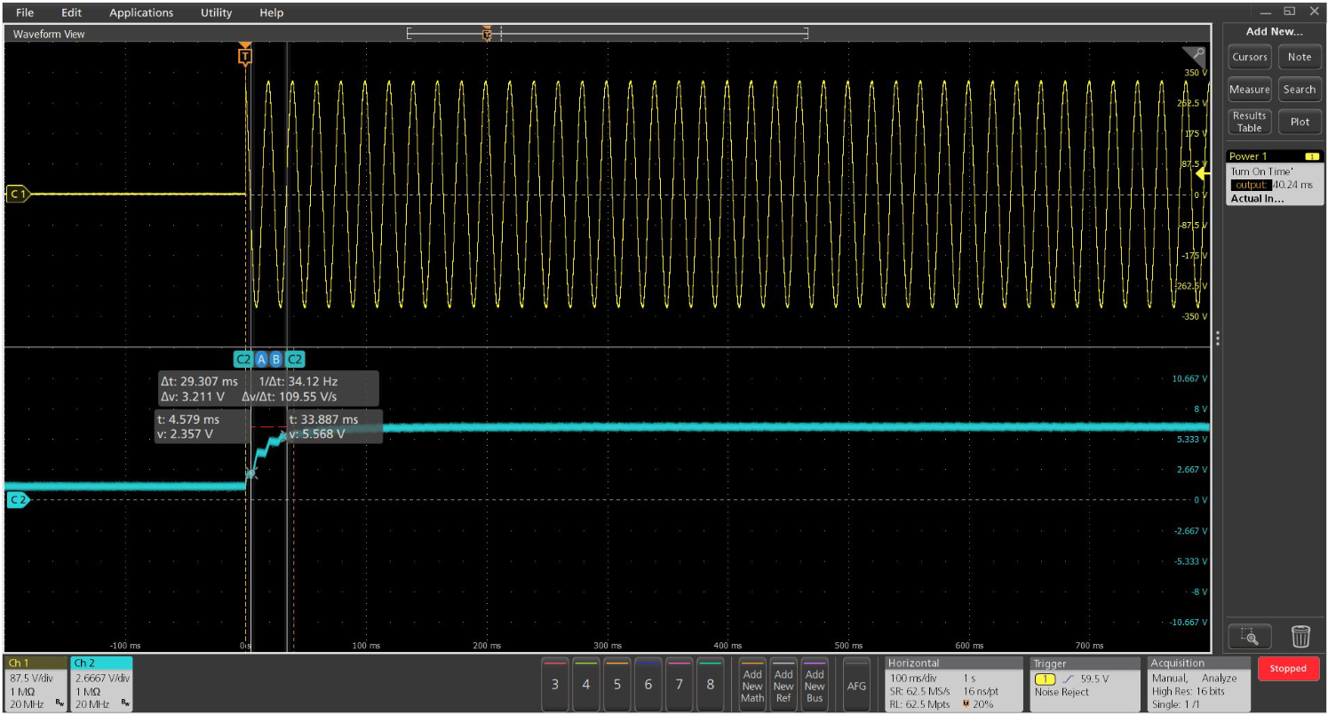
Figure 29. Turn-on time measurements find the delay between the application of input power and a stead-state output.
TURN ON TIME
Turn-On Time is the time taken to reach the output voltage of the power supply after the input voltage is applied. One channel is used to measure the input and any of the oscilloscope's remaining channels may be used to measure outputs. This enables the measurement of multiple power rails in a single acquisition.
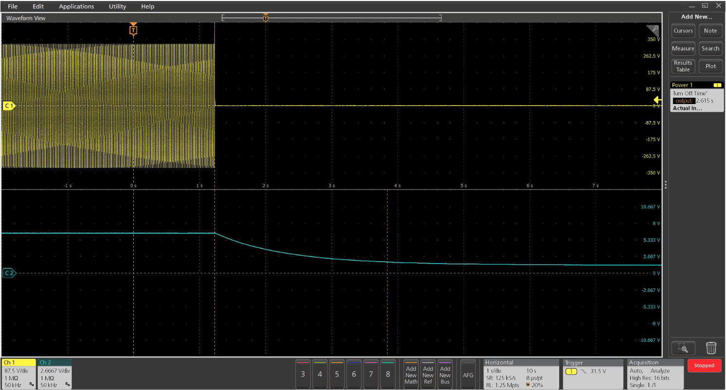
Figure 30. Turn-off time measurements find the delay between the removal of input power and a near-zero output.
TURN OFF TIME
Turn-Off Time is the time taken to get the output voltage of the power supply close to zero after the input voltage is removed.
AC to DC and DC-DC turn-on time measurements technique can be extended to verifying the power-up and power-down sequences of multiple-output supplies.
The timing and sequencing of power supply outputs during turn-on and turn-off is critical to the reliable operation of the end-products and enables devices to function without interruption. Designers will be interested to tune their end devices, say when an UPS comes back to steady state with in specified time. For example, the battery gets charged to generate DC output in a continuous manner, and the inverter system continuously charges into AC mains. If the power fails, the battery provides power to the inverter. The turn off time is important so that batter becomes active with in specified time.
Inverter Ride-Through Analysis
Grid-tie inverter systems are mandated to include anti islanding functions to prevent unintended islanding during power variations on the grid. To meet these requirements, inverter performance must be verified against international standards such as CEA, IEEE 1547, and EVS-EN 50549. These standards include ride-through timing that specifies how long a grid-tie inverter, or “smart inverter” must continue to support the grid in the event of a grid sag or overvoltage.
Power analysis software for 4, 5, and 6 Series B oscilloscopes supports automated ride-through conformance testing. Measurements can be found under Green Power Analysis and include LVRT (low voltage ride through) and HVRT (high voltage ride-through).
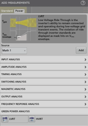
Figure 31. Green Power Analysis available in Advanced Power Measurement and Analysis Package (opt. PWR)
Both measurements rely on voltage and time masks that define “keep out” areas through which RMS voltage must not pass. The limits for these masks are defined by the standards and custom masks may also be defined.
Low voltage ride-through (LVRT) evaluates the performance of the inverter in the event of a sustained sag on the grid. The measurement is initiated when the RMS grid voltage drops below a specified level and the oscilloscope flags failures if the inverter fails to support the grid for the required time.
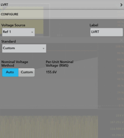
Figure 32. Setting for Low voltage ride-through measurement
Similarly, high voltage ride-through (HVRT) is a measure of inverter behavior during overvoltage grid events. The measurement identifies whether the inverter response remains within defined voltage time boundaries during these disturbances as per limits defined in the specifications.
Making the measurements
The measurement is added through the measurement panel as shown in Figure 31 and includes several parameters. This is a single-shot measurement, and the parameters help configure the scope for the sag or overvoltage event.
Specifying the test standard generates the pass/fail mask. Note that a custom mask can also be built.
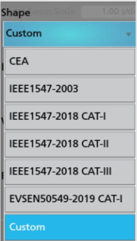
Figure 33. These standards are supported in ride-through measurements. One can also define a custom mask for margin testing or to support proprietary standards.
The nominal RMS voltage can be automatically measured by the oscilloscope or specified manually. When the Nominal Voltage Method in the measurement configuration is set to Auto, the Power Preset function captures eight cycles of the inverter’s continuous output waveform and uses them to automatically adjust the vertical and trigger settings. When the Nominal Voltage Method is set to Custom, the system does not capture the waveform; instead, it applies the vertical and trigger settings directly based on the user defined per-unit nominal voltage.

Figure 34. The default panel for the ride-through measurements. Power Preset configures the scope based on the configuration settings. The vertical scale is set according to measured voltage (Auto) or user-specified values (Custom). The selected standard determines the horizontal scale. Based on the measurement (LVRT or HVRT) the trigger is set to runt or edge with appropriate levels. Clicking the Go button sets the scope for a single shot acquisition, and it waits for a trigger.
After configuration, tapping the Power Preset button automatically selects the appropriate scale and trigger settings to acquire the intermittent grid voltage disturbance. Tapping Go arms the oscilloscope for a Single Sequence.
Measurement results
Figure 35 shows an example result for an LVRT measurement. The measurement shows the voltage and time at the first failure, and any mask hits show up in white on the RMS voltage measurement trace.
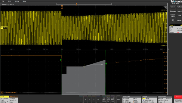
Figure 35. A low voltage ride-through failure, in which there is an RMS voltage violation. Ride-through results are displayed clearly against defined voltage time masks, making it easy to identify compliance issues. The test limits are masks defined by CEA, IEEE 1547-2003, IEEE 1547-2018 (CAT-I, CAT-II and CAT-III), EVS-EN 50549 CAT-I and Custom standards which define the boundary limit for recovery for the inverter RMS voltage. Any mask hits during the ride-through conditions fails the test.
Report Generation
Data collection, archiving and documentation are often tedious but necessary tasks in the design and development process. 4/5/6-PWR includes a report generation tool that makes the documentation of measurement results practically effortless.
By using the oscilloscope "Save as" function, a finished report with the specified layout is generated and displayed on the oscilloscope screen.
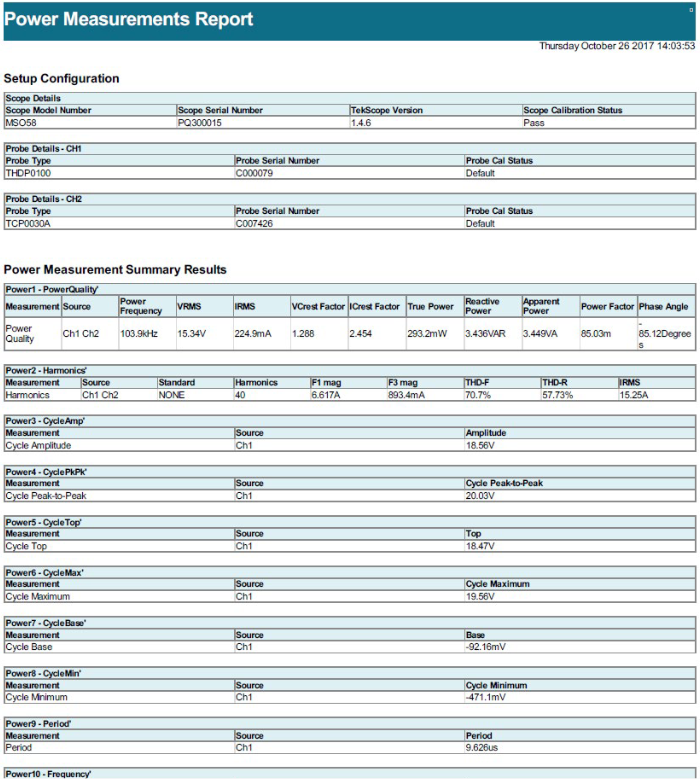
Figure 36. Reports are available in .MHT or .PDF file formats.
Summary
By using Advanced Power Measurement and Analysis options on 4, 5 and 6 Series MSO oscilloscopes, engineers can make accurate and repeatable measurements quickly and with very little setup time. Best of all, they don’t need to do manual calculations! The oscilloscope application does the work, and by using screen captures and reporting, engineers can easily provide complete documentation of how the instrument was set up, waveforms, and measurement results.
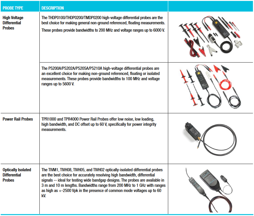
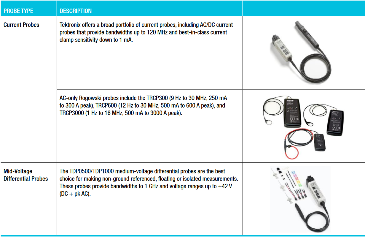
Which probes are right for your application?
4, 5 and 6 Series MSO oscilloscopes achieve the best power measurement performance when combined with the right power probes. The oscilloscopes are equipped with the TekVPI probe interface which enables communication between the oscilloscope and probes. Please refer to www.tek.com/ accessories for specific information on recommended models of differential and current probes, including IsoVu isolated probes and Rogowski probes, and any necessary probe adapters.