Why Jitter Measurement is Important
Edge jitter in serial devices is a growing concern for designers and developers. Jitter matters. It affects system performance. It is difficult to trace and characterize. And jitter limits must be met in order to comply with industry standards such as 10Gb Ethernet, PCI Express and Fibre Channel.
At the heart of the jitter measurement discipline, there is an understanding that jitter is the "canary in the coal mine1"- an advance indicator that warns of unacceptable BER performance to come. Jitter causes eye diagram openings to shrink, in turn causing receiving elements to make incorrect decisions about the state of incoming data bits and packets.
And jitter issues aren't restricted to the serial data path alone. Jitter affects timekeeping elements-clocks-as well. This too can spawn incorrect data decisions, since a misplaced clock edge can cause a data bit's state to be read too early or too late.
These are the realities of jitter. And the whole problem is compounded with each successive increase in data and clock rates. Serial bus data rates are advancing well into the multi-gigahertz range, narrowing the tolerance for any kind of timing errors. Today, measurement vendors as well as serial bus designers are investing substantial resources into research about jitter behavior. The result is a broader understanding of jitter's constituent parts and its impact on system performance. New approaches to jitter measurement are giving engineers more insight into their designs and better tools to confront the causes and effects of jitter.
1Before the advent of electronic gas-detection equipment, coal miners took caged canaries into the mine shafts to alert the workers to any accumulation of dangerous carbon monoxide in the shaft. Similarly, excessive jitter is a precursor of high BER.
This technical brief is aimed at designers, researchers, engineers, and technicians working with serial data communication architectures of all kinds. For these individuals, understanding and measuring jitter is the surest path toward solving BER problems at the system level. This document will explain some essential jitter terms, and then go on to discuss jitter measurements and the tools best suited for evaluating and quantifying jitter.
Understanding the Key Types of Jitter
Most serial communication standards specify tolerances for jitter. In addition to PCI Express, other standards that define jitter limits include SATA, SAS, USB, Infiniband, HDMI, and more. Clearly, standards committees and developers are sensitive to the problem of jitter.
Even so, some standards are surprisingly vague in their specifications. The term "jitter" actually denotes several different jitter types, some more applicable to clock signals, others more pertinent to data lines. Standards documents tend to outline quantifiable jitter limits but may not offer much guidance toward determining which type is most critical in a given application. All forms of jitter have the potential to disrupt system BER, and different tools have different strengths in detecting them.
ANSI/INCITS2 defines "timing jitter" as follows:
"The short-term variations of the significant instants of a digital signal from their ideal positions in time. Here short term implies phase oscillations of frequency greater than or equal to 10 Hz. Timing jitter may lead to crosstalk and/ or distortion of the original analog signal and is a potential source of slips at the input ports of digital switches. It may also cause slips and resultant errors in asynchronous digital multiplexers." [ANSI/INCITS T1.101-1999]
This is a good working definition of the term. But for designers attempting to make high-speed serial systems work flawlessly, it doesn't go far enough. The jitter overview in Figure 1 is not all-inclusive but it expands the definition considerably.
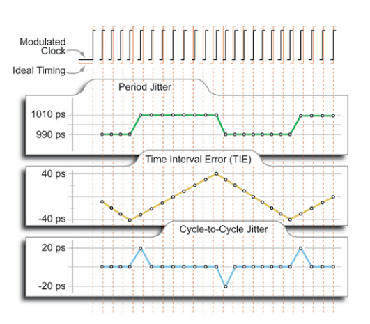
The uppermost trace in Figure 1 is a rendering of a signal waveform. The pulses shown in red are perfectly-timed "ideal" clock cycles exactly one nanosecond (1000 ps) in duration. The black traces are actual edges that exhibit jitter. Here, the trailing edges of both waveforms have been omitted to more clearly show the time-varying nature of the jitter. Note that the black rising edge shifts in time, sometimes occuring later than the red ideal edge and sometimes earlier. The left-most edge (red/black pairing) is perfectly in time. For the purposes of discussion, the measurement begins with 2nd edge, in which the black edge (the actual observed signal) occurs 10 ps early.
2ANSI: American National Standards Institute;
INCITS: International Committee for Information Technology Standards.
Each dot on the three tabbed jitter plots represents one measurement, denoting the actual placement of one edge.
The Ideal Timing waveform shows a period of exactly 1000 ps. Dashed lines have been extended through all three plots to highlight the shifts between the ideal timing and the timing of the actual measured edges.
The uppermost plot, Period Jitter. is a simple view showing period measurements of the modulated clock waveform over time. Here the period varies between 990 ps and 1010 ps. Some of the periods are 10 ps too short, followed by others that are 10 ps too long. The signal repeats this pattern.
Developers working with clock circuitry, including spreadspectrum and frequency-hopping implementations, will be most interested in period jitter. They strive for clock designs that will deliver the most accurate, predictable frequency and overall stability. Short clock periods amount to instantaneous increases in frequency, and can lead to data errors due to violation of key parameters like setup and hold timing. Obviously period jitter runs counter to this and must be measured and minimized.
Time Interval Error (TIE) Jitter is the summation of Period Jitter in a discrete fashion, period by period. The TIE plot documents the accumulating error between the ideal edge and the actual edge placement. Looking at the first four dots, or measurement points, the TIE plot tracks steadily downward (goes more negative). Each TIE point is 10 ps further away from the zero line, since the successive dots on the Period Jitter plot are each -10 ps in error. Finally when the period jitter changes from every period being short to every period being long the TIE plot "turns the corner" and heads in the positive direction after accumulating -40 ps worth of error. The TIE values are obtained by measuring the time interval from the actual edge to a reference clock.
Note that the TIE jitter value can exceed the Unit Interval (UI), a characteristic that can easily cause confusion. But the problem is readily understood if you consider that TIE can grow with every cycle. For example, if the TIE accumulates 0.1 UI in each cycle, then its value will equal 5 unit intervals after 50 cycles.
TIE measurements are useful when examining the behavior of transmitted data streams, where the reference clock is often recovered from the data signal using a phase-lock-loop (PLL). If the PLL is slow to respond to the data stream's changing bit rate, then TIE jitter will accumulate during the number of cycles it takes the PLL to catch up.
Moreover, a physical channel impairment phenomenon known as Inter-symbol Interference (ISI) can cause distorted signals. The result is "temporal spreading and consequent overlap of individual pulses to the degree that the receiver cannot reliably distinguish between changes of state" in the data stream. ISI manifests itself in the time domain as Data- Dependent Jitter (DDJ), one of the various forms of jitter included in TIE and other jitter measurements.
The Cycle-to-Cycle Jitter plot traces the dynamics of change in the clock signal. The plot depicts each cycle's change from the previous cycle. Compare the Cycle-to-Cycle with the Period Jitter plot. If there is no change from one cycle to the next, then the Cycle-to-Cycle plot line is flat. When the edge timing switches from steadily accruing error in either direction (later or earlier) the Cycle-to-Cycle plot shows the inflection point with a peak, then returns to the steadystate value. The peaks, positive or negative, occur only when there is a change in this direction.
Cycle-to-cycle jitter is useful for monitoring a clock to ensure that it does not inadvertently produce short cycles that might exceed requirements such as setup and hold timing.
Comparing Platforms for Jitter Measurement
The most common solution for acquiring and analyzing jitter is the real-time oscilloscope. Modern digitizing instruments, digital phosphor oscilloscopes (DSA/DPO), can handle today's multi-gigabit data rates. Equally important, they can be equipped with integrated software applications that perform detailed analysis of jitter and its components.
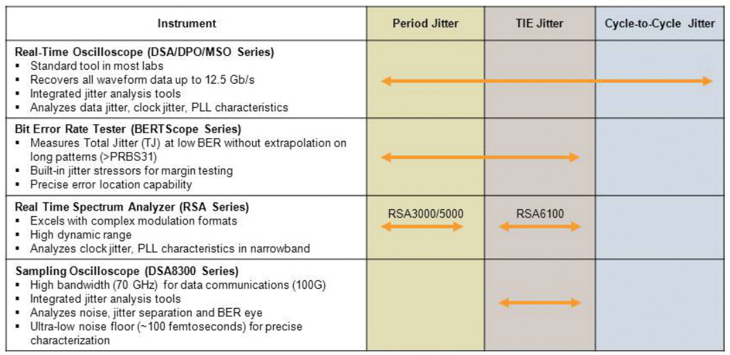
But the range of choices is not limited to DSA's and DPO's. Other entirely different platforms have their strengths, and some of their measurement capabilities overlap. Figure 2 depicts some leading jitter measurement and analysis platforms, summarizing the strengths of the various solutions in their respective application areas.
Real-Time Oscilloscopes
Because it is one of the most common measurement tools used in electronic research, development, and engineering, the real-time oscilloscope is likely to be the first line of defense when jitter issues need to be investigated. But the DSA/DPO is more than just an expedient choice; it is the ideal solution for many jitter applications and can address almost every kind of jitter measurement within reach of its bandwidth and resolution.
The DSA/DPO Real-Time Oscilloscope solution owes its jitter measurement versatility to the fact that it can capture the entire signal waveform, every detail, for many operational cycles of the DUT. Because a long history of waveform activity is preserved in the oscilloscope's sample memory, we can study attributes as varied as rise time, pulse width, and…jitter of all kinds.
High-performance DSAs can acquire uncompromised signals from many of today's leading serial buses, including Serial ATA, PCI-Express 3.0, Fibre Channel, and more. Applicable features of industry-leading DSAs include:
- 33 GHz bandwidth
- Exceptionally low jitter noise floor: <250 femtoseconds.Minimizes the oscilloscope's contribution to the DUT jitter measurement.
- 8-bit acquisition provides dynamic range sufficient for most current serial standards; suitable for 16-level modulation schemes
An equally important part of the solution is a toolset that automates jitter measurements and analysis. Jitter measurement is a rarified discipline, but one that lends itself to application-specific software solutions (assuming the oscilloscope platform supports such functions).
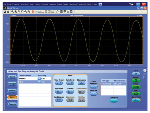
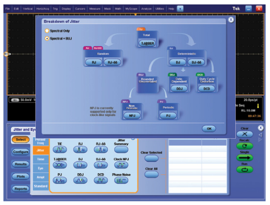
An example of this type of product is Tektronix' DPOJET Jitter and Eye measurement package. Figures 3 through 6 illustrate results obtained with this tool.

There are some applications whose demands exceed the capabilities of the real-time DSA/DPO. The instrument's realtime bandwidth and resolution must be weighed against the DUT's data rate and its harmonics. And some esoteric forms of multi-level modulation may tax the instrument's ability to distinguish between levels. In such instances, one of the other solutions will be more appropriate.
In general, though, a DSA or DPO especially when equipped with integrated analysis tools is an unsurpassed platform for jitter measurements. Because it embraces the entire continuum of jitter types, it will remain the preferred solution for most jitter analysis challenges.
Real-Time Spectrum Analyzer
Tektronix Real-Time Spectrum Analyzers (RTSA) are earning wide acceptance as general purpose frequency-domain tools and are gaining a foothold in the realm of jitter measurements.Like earlier swept spectrum analyzers, the RTSA has greater dynamic range than is available in a real-time oscilloscope.
Because the RTSA is by definition band-limited to its capture bandwidth, which in turn is processed by a resolution bandwidth (RBW) filter, the noise floor of an RTSA measurement is much lower than that of an oscilloscope. This makes the RTSA much more sensitive to low level spurious signals that are buried in the noise. If measurements such as harmonic content and low-amplitude spurious levels are required, the RTSA may be the best tool for the job.
Additionally, the phase noise of the RTSA can be several orders of magnitude better than an oscilloscope, yielding much better phase noise dynamic range for random and periodic jitter measurements. Sensitivity and phase noise dynamic range can be essential when measuring PLL and clock performance.
Current generation RTSAs such as the Tektronix RSA6100, RSA5000 and RSA3000 Series offer excellent phase measurement resolution. They can measure frequency and phase changes with greater accuracy than the same information acquired with conventional time-domain methods. This applies to jitter measurements because tiny changes in a signal's phase equate to time. When a spectrum analyzer measures jitter, it is actually measuring phase noise.
To understand that concept, consider that a signal that changes phase by 1 degree has a 1/360 change in its period. Changes in the phase of a carrier create modulation sidebands in the signal's spectrum. These sidebands can be directly measured with a spectrum analyzer. Random jitter is equivalent to the spectral phase noise floor, while periodic jitter is equivalent to all the spurs in the spectrum.
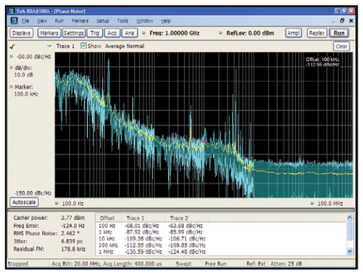
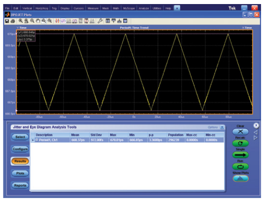
Depending on the instrument used, RTSAs can measure TIE, or Random and Periodic Jitter. In the RSA6100 Series, phase noise measurement option 10 integrates all power across the user-defined measurement bandwidth (up to 1 GHz) and calculates the Time Interval Error (see Figure 7a) in a manner similar to a swept spectrum analyzer. While RTSA do provide high precision, low residual measurements of jitter, they do not provide the rich time-domain data set available from real time oscilloscopes. Compare the single value of TIE shown in Figure 7a from the RTSA, to the statistical information available from the RT oscilloscope in Figure 7b.

While the RTSA Jitter and oscilloscope TIE Std Dev. Are in good agreement, the oscilloscope provides additional detail about the statistical nature of the signal including peak to peak, minimum and maximum TIE values. Conversely, the RTSA provides information with respect to the carrier frequency and power, RMS phase noise and residual FM present in the signal, information not available in the oscilloscope measurement.

In the RSA3000 Series with the Signal Source Analysis Suite, a part of Option 21, Random and Periodic Jitter measurements (Figure 8 below) are performed by analyzing contiguous time domain samples transformed to the frequency domain. Minimum Random Jitter measured on a 1 GHz Carrier (1 KHz to 10 MHz Bandwidth) can be as low as 0.2 picoseconds RMS. Minimum Periodic Jitter measured on the same signal is typically as low as 2 picoseconds peak excellent precision by any standard.
The RTSA makes it possible to measure the jitter on a small signal in the presence of larger ones. The unique Frequency Mask Trigger function homes in on the particular instants in time when the signal's spectrum deviates from the normal, allowing you to troubleshoot sources of jitter. Note also that an RTSA is ideally equipped to handle complex modulation schemes and other aspects of mobile voice and data transmissions. And because the RTSA has a large memory coupled with a variable effective sample rate, it can store several seconds' worth of signal activity. The RTSA is ideal for measuring random and periodic jitter in clocks and local oscillators, and for examining clock recovery systems containing PLLs and DLLs. It is less suitable for data signals and signals containing data-dependent jitter.
The RTSA has among other features the ability to capture and store a seamless, continuous record of spectral "snapshots" and process the results in many different combinations.
Real-Time Spectrum Analyzers can measure transient events and cycle-to-cycle changes, and are very useful for observing small phase variations and providing detailed views of modulation.
Sampling Oscilloscopes
The sampling oscilloscope brings prodigious bandwidth to the task of jitter measurement. At this writing, 70 GHz sampling oscilloscopes deliver unmatched signal fidelity for high-frequency time-domain measurements. A sampling oscilloscope may be the only effective solution when observing signals having data rates up to 60 Gb/s. Moreover, the sampling oscilloscope is the tool of choice when it is necessary to capture the harmonics of relatively "slow" signals. For example, a 25 Gb/s NRZ signal has a 12.5 GHz fundamental, but its 5th harmonic is 62.5 GHz--significantly beyond the reach of real-time DSA and DPO instruments today.
Sampling oscilloscopes rely on repetitive input patterns to build up a waveform acquisition made up of samples taken over numerous cycles. Many types of serial devices offer diagnostic loops that can produce these repeating waveform streams, or an external data generator can be used as a driving source.
The sampling oscilloscope has a powerful ally in the field of jitter measurements: application-specific software packages for jitter/noise analysis. The first comprehensive tool to integrate features beyond purely temporal jitter is the Tektronix 80SJNB Jitter, Noise, and BER Analysis package. Its noise analysis features set the package apart from other jitter tools on the market. Tektronix sampling oscilloscopes extend the concept of jitter analysis to encompass jitter separation, noise separation, and BER eye estimation all at bandwidths compatible with the highest serial data rates in use today.
Unifying Jitter and Noise Analysis for BER
As explained earlier this document, designers combat jitter in order to minimize its effects on BER. But jitter is only one part of the BER story it is the time, or horizontal component, of the total. A vertical component exists and plays a role in BER as well. This component is noise. A thorough jitter analysis can be done equally well with a real time oscilloscope, or an RTSA, or a sampling oscilloscope. But at this time the only solution for analyzing noise and its BER contribution is a sampling instrument.
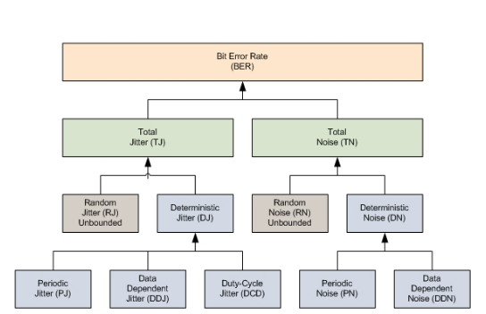
Figure 9 depicts the many factors that roll up to the total BER figure. While a detailed description of all of these factors is beyond the scope of this discussion, it is important to note that most jitter elements have counterparts on the noise side. All are made up of components that arise from both periodic and random causes within a system.
Noise is an amplitude effect that reveals itself in eye measurements. It vertically constricts the eye, closing it from above and below. Less obviously, noise also affects jitter measurements based on samples taken at a threshold crossing on an edge. The impact of these effects depends on the magnitude of the noise, the slope of the signal, and more broadly, on the transient response of the system.
In some instances, noise may be the dominant effect that degrades BER. But most often, both horizontal and vertical effects play a role in BER. Understanding the difference between noise contributions and pure jitter contributions speeds up root-cause analysis of system problems.
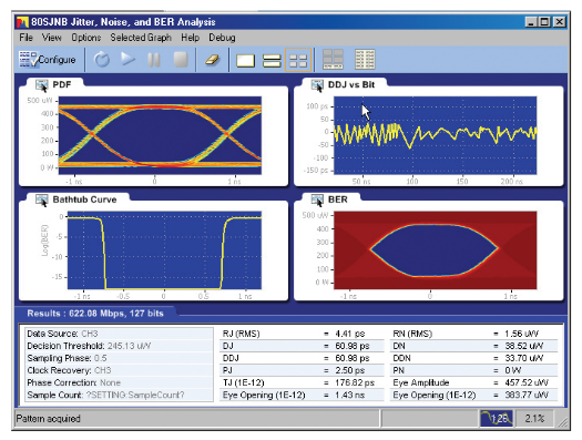
As Figure 10 shows, the sampling oscilloscope provides a wealth of information about jitter behavior, including contributions from noise. These unique views are available only through integrated jitter/noise analysis applications such as the Tektronix 80SJNB package. The Probability Distribution Function (PDF) Eye Diagram, upper left, shows the statistical probability of eye closure. The display is generated by a combination of the correlated and uncorrelated horizontal and vertical information.
Despite its similarity in appearance to conventional eye diagrams, the PDF eye is not just a plot of sample hits, and it does not close with increasing acquisition time. While the eye still is a representation of the UI of a signal digitized horizontally and vertically into a high-resolution plot, the third dimension is the calculated probability of subsequent acquisitions hitting a particular point. This probability axis is expressed by color. The PDF Eye predicts the BER outcome not by "brute force"-acquisition of vast amounts of data but by focused acquisition aimed characterizing the underlying distribution shape. Distribution after distribution is accumulated until all of the components of jitter and noise are measured and their PDFs known to a high degree of accuracy. In this way prediction of a BER of 10-18 becomes possible across the whole eye. This process provides a level of insight that would take a year to accumulate using samples on a conventional Bit Error Rate Tester (BERT).
The 2D BER Eye (lower right) is simply recalculation of the PDF Eye. Mathematically integrating the PDF yields the CDF, the Cumulative Distribution Function. This is functionally the same as the "eye contour" produced by a BERT data receiver, but there are important differences.
The sampling oscilloscope's acquisition channel delivers less than 200 femtoseconds RMS jitter while a BERT tends to be over 2x (e.g., 500 femtoseconds) the noise level. This is evidence that for very accurate timing margin characterization; a sampling scope will be an ideal choice.
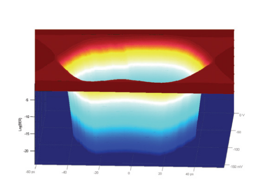
Other informative views provided by the DSA8300 Sampling Scope include the revealing 3D BER eye (Figure 11), the DDJ vs Bit plot and the bathtub curve. This latter view is especially useful for revealing the noise contribution. Tabular results are also shown. The sampling oscilloscope provides a comprehensive view of every aspect of jitter behavior. When data rates are high and it is possible to give the instrument a steady, repetitive test signal, the sampling oscilloscope is often the best solution. But because the instrument builds up a waveform record from samples acquired over many successive cycles, "single-shot" events cannot be captured. If this is not possible, then one of the other solutions may be a better choice.
BERTScope™ Bit Error Ratio Tester
Jitter for a digital communication system is defined in terms of what bit error ratio it causes. Bit Error Ratio Testers are ideal instruments for providing an accurate TJ (Total Jitter) as a result of the bit error ratio; which is a cumulative probability function. (Figure 12) That is, at a given sampling time, bit errors are the integral of all individual edges in error. This is a very important distinction because it means that in order to determine a cumulative probability using edge-timings from waveforms as the fundamental measurement, one must time a large number of edges and use software to accumulate the offending edges (thresholded by where the edge time lands too early or too late for the desired measurement instant). Alternatively, a BERT's bit decision circuit with its sampling time set to the same measurement time threshold will accumulate a count of all offending edges in real-time. In our example 10 Gbps system, in 25 μsec 250,000 bits can be counted. In one second, 10 billion bits can be counted.

With the Tektronix BERTScope, there are the algorithmic benefits of measuring real-time cumulative probability distributions with outstanding timing and decision-making fidelity to decompose jitter into its components. New jitter components, such as jitter due to intended pre-emphasis extend state-of-the-art jitter decomposition to more than just Oscilloscopes.

BERTScope has an optional Jitter Map which is a BERTbased jitter analysis engine. It has the ability to measure deep cumulative probability density functions and selectively do this for individual edges of data patterns and collections of edges. Jitter Map uses a pattern trigger, as has been key to jitter decomposition measurements made by the DSA8300 Sampling Scope. Jitter Map analysis (see Figure 13) relies on the BERTScope's error location analysis and the pattern trigger to create fast and accurate estimates reducing the need to measure all edges in a data pattern. Finally, by locking down jitter results from a shorter pattern and combining this with deep measurements of the entire pattern, jitter separation estimates can be made on very long patterns such as PRBS31. Because of the BERTScope's bit counting capability, it has the ability to identify the precise location of error patterns over long duration tests to complement TJ discoveries made by the instrument. This can provide deeper root cause insight not found in oscilloscopes or spectrum analyzers alone.
Summary: Choosing the Right Jitter Measurement Tool
Jitter measurement is a challenge that grows in importance with each advancement in system performance and data rates. There are several approaches to jitter measurement, each with its own strengths and tools. Many basic jitter tests can be handled by real-time oscilloscopes in conjunction with analysis applications that deliver both statistical and waveform information. When more dynamic range is needed, a realtime spectrum analyzer can approach jitter from a phase noise perspective, and additionally can measure jitter in the presence of interfering signals.
And when the signals in question are running at speeds beyond 40 GHz, the sampling oscilloscope is an ideal instrument for jitter measurements. With its unmatched bandwidth and its ability to parse the contribution that noise makes to BER, the sampling oscilloscope delivers unique BER insights along with its jitter measurements.
For very accurate characterization of Total Jitter using the algorithmic benefits of measuring real-time cumulative probability distributions; the BERTScope is a good fit. In addition, the BERTScope can perform advanced analysis on jitter components to enable true 10e-12 BER TJ measurements and deep insight on designs with data rates from 500 Mb/sec up to 28.6 Gb/sec.
Unsure which measurement platform is the best fit for your high-speed signal integrity challenge? Our experts can help you navigate the latest solutions and choose the right instrument with confidence.