Why a Signal Generator is Essential for Accurate Measurements
An acquisition instrument — usually an oscilloscope or logic analyzer — is probably the first thing that comes to mind when you think about making electronic measurements. But these tools can only make a measurement when they are able to acquire a signal of some kind. And there are many instances in which no such signal is available unless it is externally provided.
A strain gauge amplifier, for example, does not produce signals; it merely increases the power of the signals it receives from a sensor. Similarly, a multiplexer on a digital address bus does not originate signals; it directs signal traffic from counters, registers, and other elements. But inevitably it becomes necessary to test the amplifier or multiplexer before it is connected to the circuit that feeds it. In order to use an acquisition instrument to measure the behavior of such devices, you must provide a stimulus signal at the input.
To cite another example, engineers must characterize their emerging designs to ensure that the new hardware meets design specifications across the full range of operation and beyond. This is known as margin or limit testing. It is a measurement task that requires a complete solution; one that can generate signals as well as make measurements. The toolset for digital design characterization differs from its counterpart in analog/mixed signal design, but both must include stimulus instruments and acquisition instruments.
The signal generator, or signal source, is the stimulus source that pairs with an acquisition instrument to create the two elements of a complete measurement solution. The two tools flank the input and output terminals of the device-under-test (DUT) as shown in Figure 1. In its various configurations, the signal generator can provide stimulus signals in the form of analog waveforms, digital data patterns, modulation, intentional distortion, noise, and more. To make effective design, characterization, or troubleshooting measurements, it is important to consider both elements of the solution.
The purpose of this document is to explain signal generators, their contribution to the measurement solution as a whole and their applications. Understanding the many types of signal generators and their capabilities is essential to your work as a researcher, engineer or technician. Selecting the right tool will make your job easier and will help you produce fast, reliable results.
After reading this primer, you will be able to:
- Describe how signal generators work
- Describe electrical waveform types
- Describe the differences between mixed signal generators and logic signal generators
- Understand basic signal generator controls
- Generate simple waveforms
Should you need additional assistance, or have any comments or questions about the material in this primer, simply contact your Tektronix representative, or visit https://www.tek.com/products/signal-generators.
Introduction to Signal Generators
The signal generator is exactly what its name implies: a generator of signals used as a stimulus for electronic measurements. Most circuits require some type of input signal whose amplitude varies over time. The signal may be a true bipolar AC1 signal (with peaks oscillating above and below a ground reference point) or it may vary over a range of DC offset voltages, either positive or negative. It may be a sine wave or other analog function, a digital pulse, a binary pattern or a purely arbitrary wave shape.
The signal generator can provide "ideal" waveforms or it may add known, repeatable amounts and types of distortion (or errors) to the signal it delivers. See Figure 2. This characteristic is one of the signal generator's greatest virtues, since it is often impossible to create predictable distortion exactly when and where it's needed using only the circuit itself. The response of the DUT in the presence of these distorted signals reveals its ability to handle stresses that fall outside the normal performance envelope.
Analog or Digital?
Most signal generators today are based on digital technology. Many can fulfill both analog and digital requirements, although the most efficient solution is usually a source whose features are optimized for the application at hand — either analog or digital.
Arbitrary waveform generators (AWG) and function generators are aimed primarily at analog and mixed-signal applications. These instruments use sampling techniques to build and modify waveforms of almost any imaginable shape. Typically these generators have from 1 to 4 outputs. In some AWGs, these main sampled analog outputs are supplemented by separate marker outputs (to aid triggering of external instruments) and synchronous digital outputs that present sample-by-sample data in digital form.
Digital waveform generators (logic sources) encompass two classes of instruments. Pulse generators drive a stream of square waves or pulses from a small number of outputs, usually at very high frequencies. These tools are most commonly used to exercise high-speed digital equipment. Pattern generators, also known as data generators or data timing generators, typically provide 8, 16, or even more synchronized digital pulse streams as a stimulus signal for computer buses, digital telecom elements, and more.
Basic Signal Generator Applications
Signal generators have hundreds of different applications but in the electronic measurement context they fall into three basic categories: verification, characterization, and stress/margin testing. Some representative applications include:
Verification
Testing Digital Modular Transmitters and Receivers
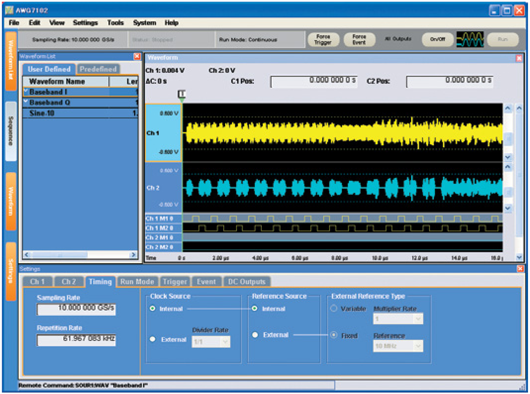
Wireless equipment designers developing new transmitter and receiver hardware must simulate baseband I&Q signals — with and without impairments — to verify conformance with emerging and proprietary wireless standards. Some high-performance arbitrary waveform generators can provide the needed lowdistortion, high-resolution signals at rates up to 12.5Gb/s, with two independent channels, one for the "I" phase and one for the "Q" phase.
Sometimes the actual RF signal is needed to test a receiver. In this case, arbitrary waveform generators with Output Frequencies up to 20 GHz can be used to directly synthesize the RF signal.
Characterization
Testing D/A and A/D Converters
Newly-developed digital-to-analog converters (DAC) and analogto- digital converters (ADC) must be exhaustively tested to determine their limits of linearity, monotonicity, and distortion. A state-of-the-art AWG can generate simultaneous, in-phase analog and digital signals to drive such devices at speeds up to 12.5Gb/s.
Stress/Margin Testing
Stressing Communication Receivers
Engineers working with serial data stream architectures (commonly used in digital communications buses and disk drive amplifiers) need to stress their devices with impairments, particularly jitter and timing violations. Advanced signal generators save the engineer untold hours of calculation by providing efficient built-in jitter editing and generation tools. These instruments can shift critical signal edges as little as 20ps.
Signal Generation Techniques
There are several ways to create waveforms with a signal generator. The choice of methods depends upon the information available about the DUT and its input requirements; whether there is a need to add distortion or error signals, and other variables. Modern high-performance signal generators offer at least three ways to develop waveforms:
- Create: Brand new signals for circuit stimulus and testing
- Replicate: Synthesize an unavailable real-world signal (captured from an oscilloscope or logic analyzer)
- Generate: Ideal or stressed reference signals for industry standards with specific tolerances
Understanding Signal Generator Waveforms
Waveform Characteristics
The term "wave" can be defined as a pattern of varying quantitative values that repeats over some interval of time. Waves are common in nature: sound waves, brain waves, ocean waves, light waves, voltage waves, and many more. All are periodically repeating phenomena. Signal generators are usually concerned with producing electrical (typically voltage) waves that repeat in a controllable manner.
Each full repetition of a wave is known as a "cycle." A waveform is a graphic representation of the wave's activity — its variation over time. A voltage waveform is a classic Cartesian graph with time on the horizontal axis and voltage on the vertical axis. Note that some instruments can capture or produce current waveforms, power waveforms, or other alternatives. In this document we will concentrate on the conventional voltage vs. time waveform.
Amplitude, Frequency, and Phase
Waveforms have many characteristics but their key properties pertain to amplitude, frequency, and phase:
- Amplitude: A measure of the voltage "strength" of the waveform. Amplitude is constantly changing in an AC signal. Signal generators allow you to set a voltage range, for example, —3 to +3 volts. This will produce a signal that fluctuates between the two voltage values, with the rate of change dependent upon both the wave shape and the frequency.
- Frequency: The rate at which full waveform cycles occur. Frequency is measured in Hertz (Hz), formerly known as cycles per second. Frequency is inversely related to the period (or wavelength) of the waveform, which is a measure of the distance between two similar peaks on adjacent waves. Higher frequencies have shorter periods.
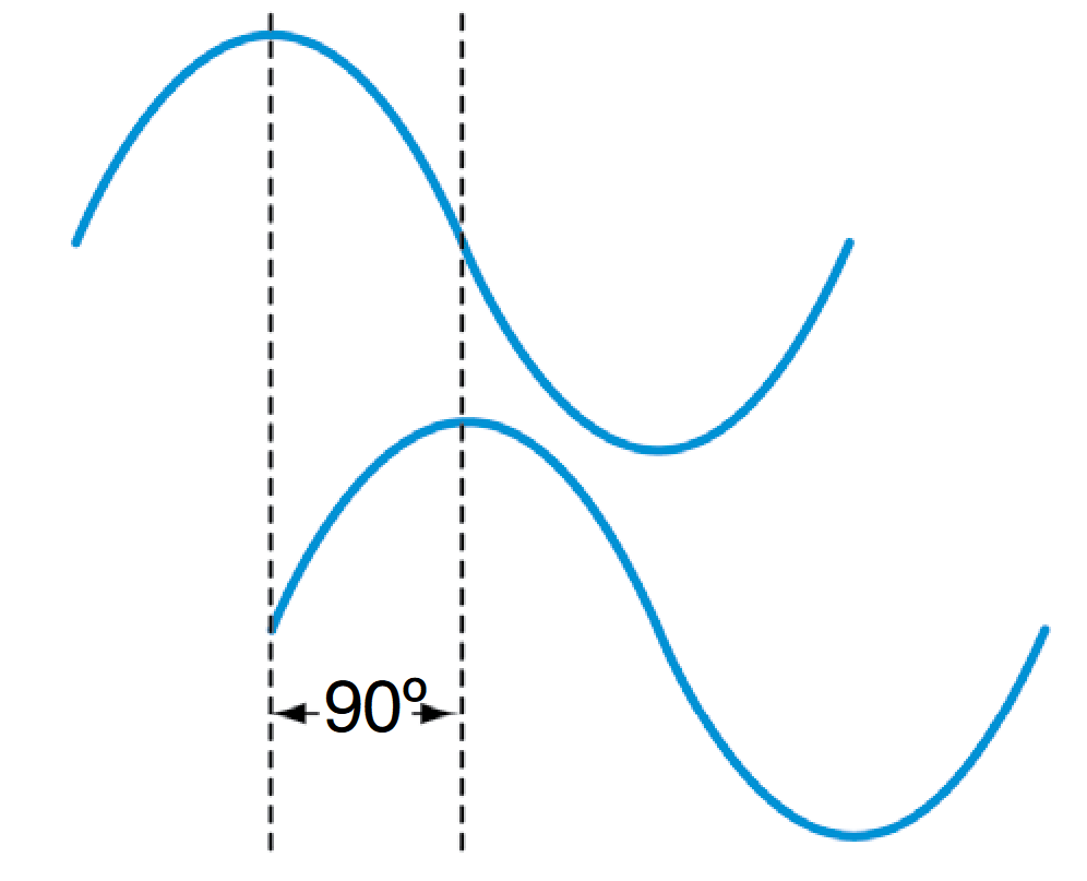
- Phase: In theory, the placement of a waveform cycle relative to a 0 degree point. In practice, phase is the time placement of a cycle relative to a reference waveform or point in time.
Phase is best explained by looking at a sine wave. The voltage level of sine waves is mathematically related to circular motion. Like a full circle, one cycle of a sine wave travels through 360 degrees. The phase angle of a sine wave describes how much of its period has elapsed.
Two waveforms may have identical frequency and amplitude and still differ in phase. Phase shift, also known as delay, describes the difference in timing between two otherwise similar signals, as shown in Figure 4. Phase shifts are common in electronics.
The amplitude, frequency, and phase characteristics of a waveform are the building blocks a signal generator uses to optimize waveforms for almost any application. In addition, there are other parameters that further define signals, and these too are implemented as controlled variables in many signal generators.
Rise and Fall Time
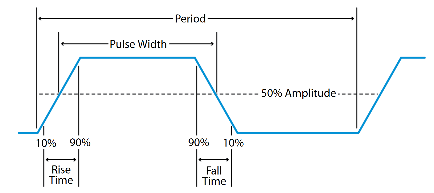
Edge transition times, also referred to as rise and fall times, are characteristics usually ascribed to pulses and square waves. They are measures of the time it takes the signal edge to make a transition from one state to another. In modern digital circuitry, these values are usually in the low nanosecond range or less.
Both rise and fall times are measured between the 10% and 90% points of the static voltage levels before and after the transition (20% and 80% points are sometimes used as alternatives). Figure 5 illustrates a pulse and some of the characteristics associated with it. This is an image of the type you would see on an oscilloscope set at a high sample rate relative to the frequency of the incoming signal. At a lower sample rate, this same waveform would look much more "square."
In some cases, rise and fall times of generated pulses need to be varied independently, for example when using generated pulses to measure an amplifier with unsymmetrical slew rates, or controlling the cool down time of a laser spot welding gun.
Pulse Width
Pulse width is the time that elapses between the leading and trailing edges of a pulse. Note that the term "leading" applies to either positive-going or negative-going edges as does the term "trailing." In other words, these terms denote the order in which the events occur during a given cycle; a pulse's polarity does not affect its status as the leading or trailing edge. In Figure 5, the positive-going edge is the leading edge. The pulse width measurement expressed the time between the 50% amplitude points of the respective edges.
To cite a tangible example of a duty cycle, imagine an actuator that must rest for three seconds after each one-second burst of activity, in order to prevent the motor from overheating. The actuator rests for three seconds out of every four — a 25% duty cycle.
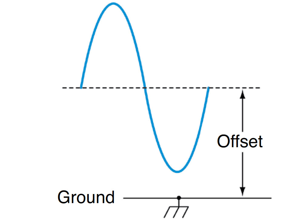
Offset
Not all signals have their amplitude variations centered on a ground (0 V) reference. The "offset" voltage is the voltage between circuit ground and the center of the signal's amplitude. In effect, the offset voltage expresses the DC component of a signal containing both AC and DC values, as shown in Figure 6.
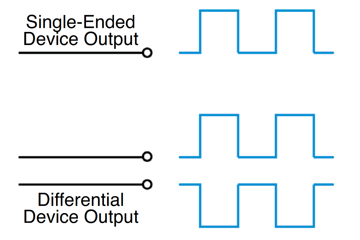
Differential vs. Single-ended
Signals Differential signals are those that use two complementary paths carrying copies of the same signal in equal and opposite polarity (relative to ground). As the signal's cycle proceeds and the one path becomes more positive, the other becomes more negative to the same degree. For example, if the signal's value at some instant in time was +1.5 volts on one of the paths, then the value on the other path would be exactly -1.5 volts (assuming the two signals were perfectly in phase). The differential architecture is good at rejecting crosstalk and noise and passing only the valid signal.
Single-ended operation is a more common architecture, in which there is only one path plus ground. Figure 7 illustrates both single-ended and differential approaches.
Basic Waves
Waveforms come in many shapes and forms. Most electronic measurements use one or more of the following wave shapes, often with noise or distortion added:
- Sine waves
- Square and rectangular waves
- Sawtooth and triangle waves
- Step and pulse shapes
- Complex waves
Sine Waves
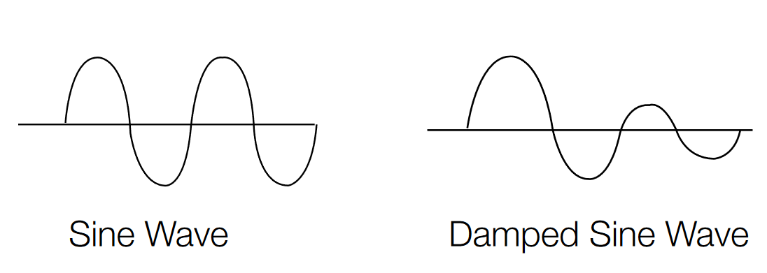
Sine waves are perhaps the most recognizable wave shape. Most AC power sources produce sine waves. Household wall outlets deliver power in the form of sine waves. And the sine wave is almost always used in elementary classroom demonstrations of electrical and electronic principles. The sine wave is the result of a basic mathematical function — graphing a sine curve through 360 degrees will produce a definitive sine wave image.
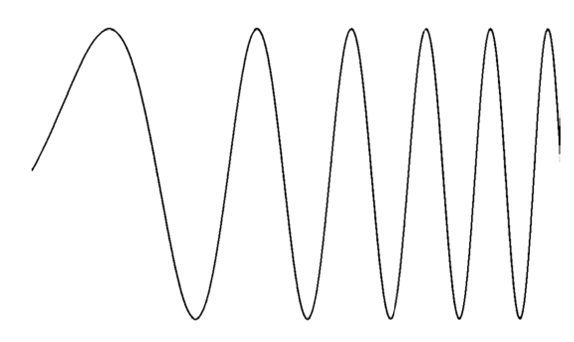
The damped sine wave is a special case in which a circuit oscillates from an impulse, and then winds down over time.
Figure 8 shows examples of sine and damped sine wavederived signals.
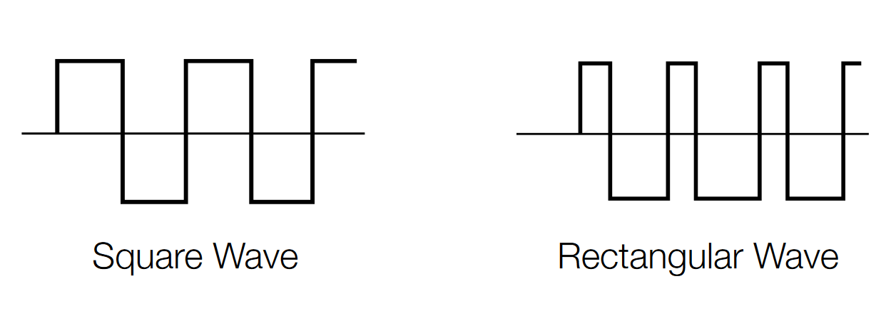
Square and Rectangular Waves
Square and rectangular waves are basic forms that are at the heart of all digital electronics, and they have other uses as well. A square wave is a voltage that switches between two fixed voltage levels at equal intervals. It is routinely used to test amplifiers, which should be able to reproduce the fast transitions between the two voltage levels (these are the rise and fall times explained earlier). The square wave makes an ideal timekeeping clock for digital systems — computers, wireless telecom equipment, HDTV systems, and more.
A rectangular wave has switching characteristics similar to those of a square wave, except that its high and low time intervals are not of equal length, as described in the earlier "duty cycle" explanation. Figure 9 shows examples of square and rectangular waves.
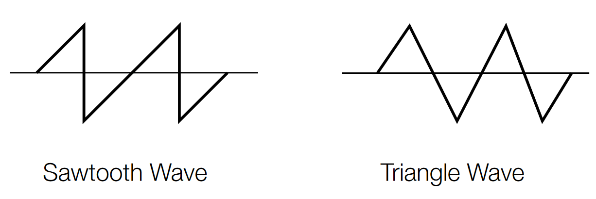
Sawtooth and Triangle Waves
Sawtooth and triangle waves look very much like the geometric shapes they are named for. The sawtooth ramps up slowly and evenly to a peak in each cycle, then falls off quickly. The triangle has more symmetrical rise and fall times. These waveforms are often used to control other voltages in systems such as analog oscilloscopes and televisions. Figure 10 shows examples of sawtooth and triangle waves.
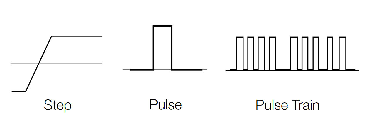
Step and Pulse Shapes
A "step" is simply a waveform that shows a sudden change in voltage, as though a power switch had been turned on.
The "pulse" is related to the rectangular wave. Like the rectangle, it is produced by switching up and then down, or down and then up, between two fixed voltage levels. Pulses are inherently binary and therefore are the basic tool for carrying information (data) in digital systems. A pulse might represent one bit of information traveling through a computer. A collection of pulses traveling together creates a pulse train. A synchronized group of pulse trains (which may be transmitted in parallel or serial fashion) makes up a digital pattern. Figure 11 shows examples of step and pulse shapes and a pulse train.
Note that, while digital data is nominally made up of pulses, rectangles, and square waves, real-world digital waveforms exhibit more rounded corners and slanted edges.
Sometimes, circuit anomalies produce pulses spontaneously. Usually these transient signals occur non-periodically, and have come to be described with the term "glitch." One of the challenges of digital troubleshooting is distinguishing glitch pulses from valid but narrow data pulses. And one of the strengths of certain types of signal generators is their ability to add glitches anywhere in a pulse train.
Complex Waves
In operational electronic systems, waveforms rarely look like the textbook examples explained above. Certain clock and carrier signals are pure, but most other waveforms will exhibit some unintended distortion (a by-product of circuit realities like distributed capacitance, crosstalk, and more) or deliberate modulation. Some waveforms may even include elements of sines, squares, steps, and pulses.
Complex waves include:
- Analog modulated, digitally modulated, pulse-width modulated, and quadrature modulated signals
- Digital patterns and formats
- Pseudo-random bit and word streams
Signal Modulation
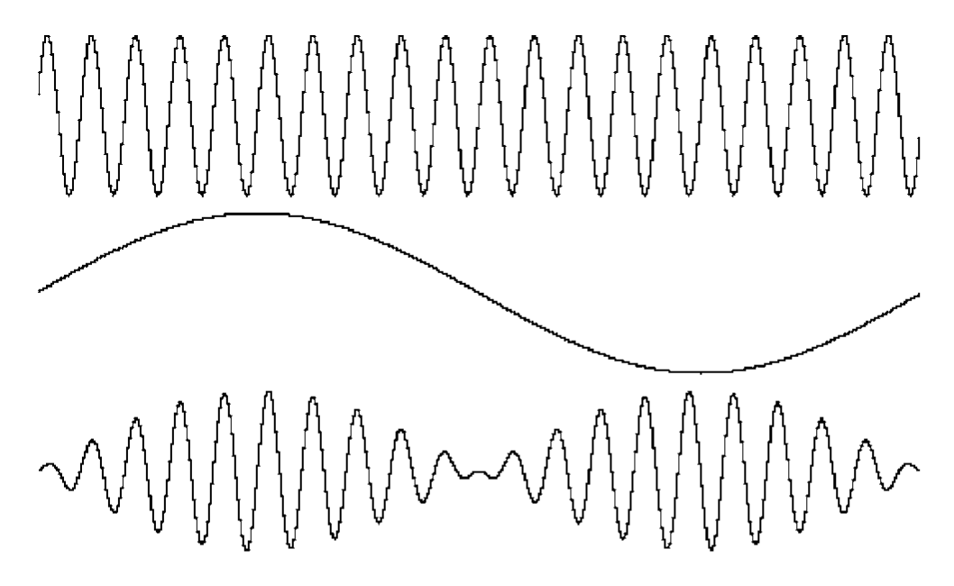
In modulated signals, amplitude, phase and/or frequency variations embed lower-frequency information into a carrier signal of higher frequency. The resulting signals may convey anything from speech to data to video. The waveforms can be a challenge to reproduce unless the signal generator is specifically equipped to do so.
Analog Modulation. Amplitude modulation (AM) and frequency modulation (FM) are most commonly used in broadcast communications. The modulating signal varies the carrier's amplitude and/or frequency. At the receiving end, demodulating circuits interpret the amplitude and/or frequency variations, and extract the content from the carrier.
Phase modulation (PM) modulates the phase rather than the frequency of the carrier waveform to embed the content.
Figure 12 illustrates an example of analog modulation.
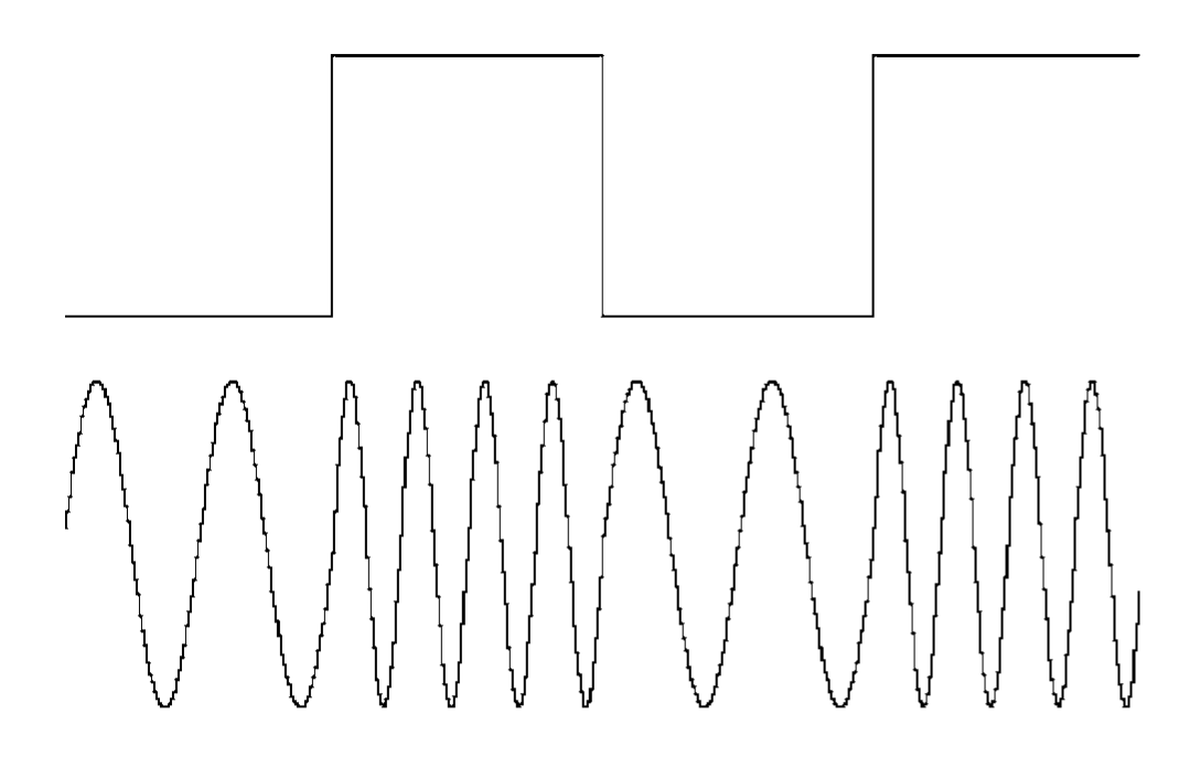
Digital Modulation. Digital modulation, like other digital technologies, is based on two states which allow the signal to express binary data. In amplitude-shift keying (ASK), the digital modulating signal causes the output frequency to switch between two amplitudes; in frequency-shift keying (FSK), the carrier switches between two frequencies (its center frequency and an offset frequency); and in phase-shift keying (PSK), the carrier switches between two phase settings. In PSK, a "0" is imparted by sending a signal of the same phase as the previous signal, while a "1" bit is represented by sending a signal of the opposite phase.
Pulse-width modulation (PWM) is yet another common digital format; it is often used in digital audio systems. As its name implies, it is applicable to pulse waveforms only. With PWM, the modulating signal causes the active pulse width (duty cycle, explained earlier) of the pulse to vary.
Figure 13 shows an example of digital modulation.
Frequency Sweep
Measuring the frequency characteristics of an electronic device calls for a "swept" sine wave — one that changes in frequency over a period of time. The frequency change occurs linearly in "Hz per seconds" or logarithmically in "Octaves per second." Advanced sweep generators support sweep sequences with selectable start frequency, hold frequency, stop frequency and associated times. The signal generator also provides a trigger signal synchronously to the sweep to control an oscilloscope that measures the output response of the device.
Quadrature Modulation. Today's digital wireless communications networks are built on a foundation of quadrature (IQ) modulation technology. Two carriers — an inphase (I) waveform and a quadrature-phase (Q) waveform that is delayed by exactly 90 degrees relative to the "I" waveform — are modulated to produce four states of information. The two carriers are combined and transmitted over one channel, then separated and demodulated at the receiving end. The IQ format delivers far more information than other forms of analog and digital modulation: it increases the effective bandwidth of the system. Figure 15 depicts quadrature modulation.
Digital Patterns and Formats
A digital pattern consists of multiple synchronized pulse streams that make up "words" of data that may be 8, 12, 16, or more bits wide. One class of signal generator, the digital pattern generator, specializes in delivering words of data to digital buses and processors via parallel outputs. The words in these patterns are transmitted in a steady march of cycles, with the activity for each bit in each cycle determined by the chosen signal format. The formats affect the width of the pulses within the cycles that compose the data streams.
The following list summarizes the most common signal formats. The first three format explanations assume that the cycle begins with a binary "0" value – that is, a low logic voltage level.
- Non-Return-to-Zero (NRZ): When a valid bit occurs in the cycle, the waveform switches to a "1" and stays at that value until the next cycle boundary.
- Delayed Non-Return-to-Zero (DNRZ): Similar to NRZ, except that the waveform switches to a "1" after a specified delay time.
- Return-to-Zero (RZ): When a valid bit is present, the waveform switches to a "1," then back to a "0" within the same cycle.
- Return-to-One (R1): In effect, the inverse of RZ. Unlike the other formats in this list, R1 assumes the cycle begins with a "1", then switches to a "0" when the bit is valid, then switches back to a "1" before the cycle ends.
Bit Streams
Pseudo-random bit sequence (PRBS) and pseudo-random word sequence (PRWS) exist to make up for an innate limitation in digital computers: their inability to produce truly random numbers. Yet random events can have beneficial uses in digital systems. For example, perfectly "clean" digital video signals may have objectionable jagged lines and noticeable contours on surfaces that should be smooth. Adding a controlled amount of noise can hide these artifacts from the eye without compromising the underlying information.
To create random noise, digital systems produce a stream of numbers that has the effect of randomness even though the numbers follow a predictable mathematical pattern. These "pseudo-random" numbers are actually a set of sequences repeated at a random rate. The result is a PRBS. A pseudorandom word stream defines how multiple PRBS streams are presented across the signal generator's parallel outputs.
PRWS is often used when testing serializers or multiplexers. These elements reassemble the PRWS signal into a serial stream of pseudo-random bits.
Types of Signal Generators
Broadly divided into mixed signal generators (arbitrary waveform generators and arbitrary/function generators) and logic sources (pulse or pattern generators), signal generators span the whole range of signal-producing needs. Each of these types has unique strengths that may make it more or less suitable for specific applications.
Mixed signal generators are designed to output waveforms with analog characteristics. These may range from analog waves such as sines and triangles to "square" waves that exhibit the rounding and imperfections that are part of every real-world signal. In a versatile mixed signal generator, you can control amplitude, frequency, and phase as well as DC offset and rise and fall time; you can create aberrations such as overshoot; and you can add edge jitter, modulation and more.
True digital sources are meant to drive digital systems. Their outputs are binary pulse streams – a dedicated digital source cannot produce a sine or triangle wave. The features of a digital source are optimized for computer bus needs and similar applications. These features might include software tools to speed pattern development as well as hardware tools such as probes designed to match various logic families.
As explained earlier, almost all high-performance signal generators today, from function generators to arbitrary sources to pattern generators, are based on digital architectures, allowing flexible programmability and exceptional accuracy.
Analog and Mixed Signal Generators
Types of Analog and Mixed Signal Generators
Arbitrary Generators
Historically, the task of producing diverse waveforms has been filled by separate, dedicated signal generators, from ultra-pure audio sine wave generators to multi-GHz RF signal generators. While there are many commercial solutions, the user often must custom-design or modify a signal generator for the project at hand. It can be very difficult to design an instrumentationquality signal generator, and of course, the time spent designing ancillary test equipment is a costly distraction from the project itself.
Fortunately, digital sampling technology and signal processing techniques have brought us a solution that answers almost any kind of signal generation need with just one type of instrument – the arbitrary generator. Arbitrary generators can be classified into arbitrary/function generators (AFG) and arbitrary waveform generators (AWG).
Arbitrary/Function Generator (AFG)
The arbitrary/function generator (AFG) serves a wide range of stimulus needs; in fact, it is the prevailing signal generator architecture in the industry today. Typically, this instrument offers fewer waveform variations than its AWG equivalent, but with excellent stability and fast response to frequency changes. If the DUT requires the classic sine and square waveforms (to name a few) and the ability to switch almost instantly between two frequencies, the arbitrary/function generator (AFG) is the right tool. An additional virtue is the AFG's low cost, which makes it very attractive for applications that do not require an AWG's versatility.
The AFG shares many features with the AWG, although the AFG is by design a more specialized instrument. The AFG offers unique strengths: it produces stable waveforms in standard shapes – particularly the all-important sine and square waves – that are both accurate and agile. Agility is the ability to change quickly and cleanly from one frequency to another.
Most AFGs offer some subset of the following familiar wave shapes:
- Sine
- Square
- Triangle
- Sweep
- Pulse
- Ramp
- Modulation
- Haversine
While AWGs can certainly provide these same waveforms, today's AFGs are designed to provide improved phase, frequency, and amplitude control of the output signal. Moreover, many AFGs offer a way to modulate the signal from internal or external sources, which is essential for some types of standards compliance testing.
In the past, AFGs created their output signals using analog oscillators and signal conditioning. More recent AFGs rely on Direct Digital Synthesis (DDS) techniques to determine the rate at which samples are clocked out of their memory.
DDS technology synthesizes waveforms by using a single clock frequency to spawn any frequency within the instrument's range. Figure 16 summarizes the DDS-based AFG architecture in simplified form.
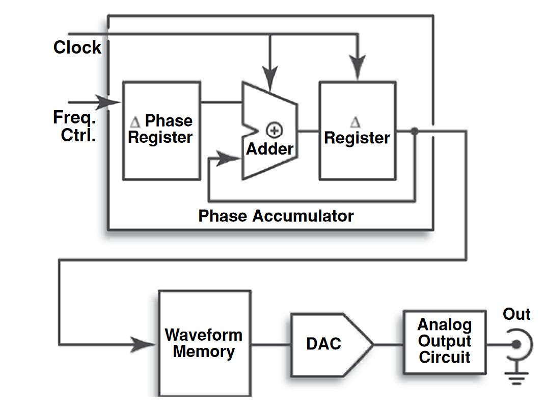
In the phase accumulator circuit, the Delta (D) phase register receives instructions from a frequency controller, expressing the phase increments by which the output signal will advance in each successive cycle. In a modern high-performance AFG, the phase resolution may be as small as one part in 230, that is, approximately 1/1,000,000,000.
The output of the phase accumulator serves as the clock for the waveform memory portion of the AFG. The instrument's operation is almost the same as that of the AWG, with the notable exception that the waveform memory typically contains just a few basic signals such as sine and square waves. The analog output circuit is basically a fixed-frequency, low-pass filter which ensures that only the programmed frequency of interest (and no clock artifacts) leaves the AFG output.
To understand how the phase accumulator creates a frequency, imagine that the controller sends a value of 1 to the 30-bit D phase register. The phase accumulator's D output register will advance by 360 ÷ 230 in each cycle, since 360 degrees represents a full cycle of the instrument's output waveform. Therefore, a D phase register value of 1 produces the lowest frequency waveform in the AFG's range, requiring the full 2D increments to create one cycle. The circuit will remain at this frequency until a new value is loaded into the D phase register.
Values greater than 1 will advance through the 360 degrees more quickly, producing a higher output frequency (some AFGs use a different approach: they increase the output frequency by skipping some samples, thereby reading the memory content faster). The only thing that changes is the phase value supplied by the frequency controller. The main clock frequency does not need to change at all. In addition, it allows a waveform to commence from any point in the waveform cycle.
For example, assume it is necessary to produce a sine wave that begins at the peak of the positive-going part of the cycle. Basic math tells us that this peak occurs at 90 degrees. Therefore:
230 increments = 360¡ ; and
90¡ = 360¡ ÷ 4; then,
90¡ = 230 ÷ 4
When the phase accumulator receives a value equivalent to (230 ÷ 4), it will prompt the waveform memory to start from a location containing the positive peak voltage of the sine wave.
The typical AFG has several standard waveforms stored in a preprogrammed part of its memory. In general, sine and square waves are the most widely used for many test applications. Arbitrary waveforms are held in a user programmable part of the memory. Waveshapes can be defined with the same flexibility as in conventional AWGs. However, the DDS architecture does not support memory segmentation and waveform sequencing. These advanced capabilities are reserved for high performance AWGs.
DDS architecture provides exceptional frequency agility, making it easy to program both frequency and phase changes on the fly, which is useful to test any type of FM DUT – radio and satellite system components, for example. And if the specific AFG's frequency range is sufficient, it's an ideal signal generator for test on FSK and frequency-hopping telephony technologies such as GSM.
Although it cannot equal the AWG's ability to create virtually any imaginable waveform, the AFG produces the most common test signals used in labs, repair facilities and design departments around the world. Moreover, it delivers excellent frequency agility. And importantly, the AFG is often a very costeffective way to get the job done.
Arbitrary Waveform Generator (AWG)
Whether you want a data stream shaped by a precise Lorentzian pulse for disk drive characterization, or a complex modulated RF signal to test a GSM- or CDMA-based telephone handset, the arbitrary waveform generator (AWG) can produce any waveform you can imagine. You can use a variety of methods – from mathematical formulae to "drawing" the waveform – to create the needed output.
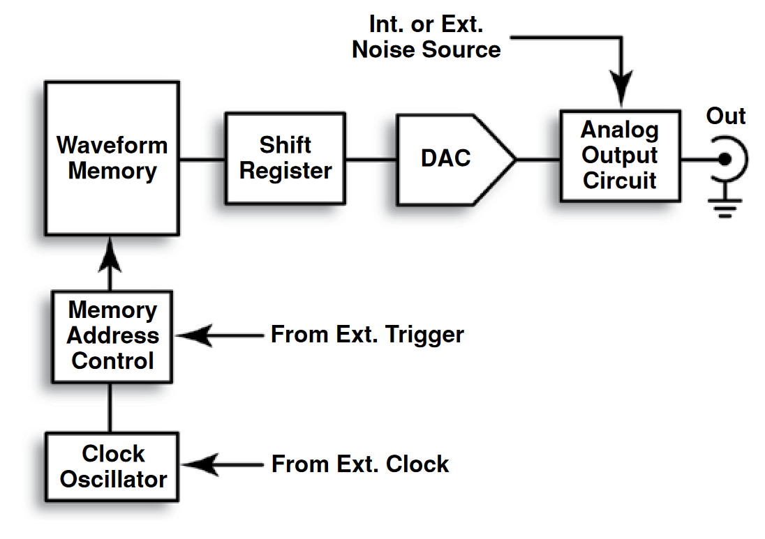
Fundamentally, an arbitrary waveform generator (AWG) is a sophisticated playback system that delivers waveforms based on stored digital data that describes the constantly changing voltage levels of an AC signal. It is a tool whose block diagram is deceptively simple. To put the AWG concept in familiar terms, it is much like a CD player that reads out stored data (in the AWG, its own waveform memory; in the CD player, the disc itself) in real time. Both put out an analog signal, or waveform.
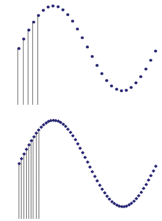
To understand the AWG, it's first necessary to grasp the broad concepts of digital sampling. Digital sampling is exactly what its name implies: defining a signal using samples, or data points, that represent a series of voltage measurements along the slope of the waveform. These samples may be determined by actually measuring a waveform with an instrument such as an oscilloscope, or by using graphical or mathematical techniques. Figure 17 (Left) depicts a series of sampled points. All of the points are sampled at uniform time intervals, even though the curve makes their spacing appear to vary. In an AWG, the sampled values are stored in binary form in a fast Random Access Memory (RAM).
With the stored information, the signal can be reconstructed (bottom) at any time by reading back the memory locations and feeding the data points through a digital-to-analog converter (DAC). Figure 17 (Right) depicts the result. Note that the AWG's output circuitry filters between the points to connect the dots and create a clean, uninterrupted waveform shape. The DUT does not "see" these dots as discrete points, but as a continuous analog waveform.
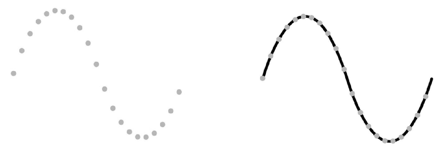
Figure 18 is a simplified block diagram of an AWG that implements these operations.
The AWG offers a degree of versatility that few instruments can match. With its ability to produce any waveform imaginable, the AWG embraces applications ranging from automotive anti-lock brake system simulation to wireless network stress testing.
How to use a Signal Generator
The Systems and Controls of a Mixed Signal Generator
Consistent with its role as the stimulus element of a complete measurement solution, the mixed-signal generator's controls and subsystems are designed to speed the development of a wide range of waveform types, and to deliver the waveforms with uncompromised fidelity.
The most basic and frequently-manipulated signal parameters have their own dedicated front-panel controls. More complex operations and those that are needed less frequently are accessed via menus on the instrument's display screen.
The Level Control is responsible for setting the amplitude and offset level of the output signal. In the signal generator depicted in Figure 19, the dedicated level controls on the front panel make it easy to set amplitude and offset values without relying on multi-level menus.
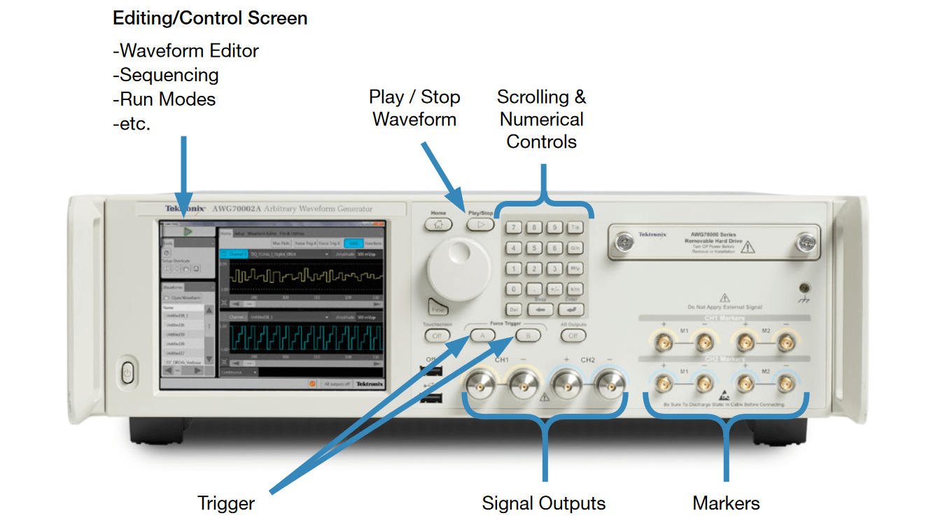
The Timing Control sets the frequency of the output signal by controlling the sample rate. Here, too, dedicated hardwarebased controls simplify setup of the essential horizontal parameters.
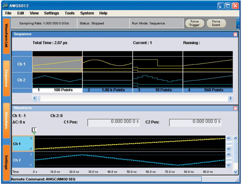
Note that none of the parameters above control the actual wave shape that the instrument produces. This functionality resides in menus on the Editing/Control Screen. The touch panel or mouse selects the view of interest, which might offer controls to define sequences, or digital output settings in the graphical user interface as shown in Figure 20. After bringing up such a page, you simply fill in the blanks using the numerical keypad and/or the general-purpose scrolling knob.
Performance Terms and Considerations
Following are some definitions of parameters that describe the performance of a mixed signal generator. You will see these terms used in brochures, reference books, tutorials almost anywhere signal generators or their applications are described.
Memory Depth (Record Length)
Memory depth, or record length, goes hand-in-hand with clock frequency. Memory depth determines the maximum number of samples that can be stored. Every waveform sample point occupies a memory location. Each location equates to a sample interval's worth of time at the current clock frequency. If the clock is running at 100 MHz, for example, the stored samples are separated by 10 ns.
Memory depth plays an important role in signal fidelity at many frequencies because it determines how many points of data can be stored to define a waveform. Particularly in the case of complex waveforms, memory depth is critical to reproducing signal details accurately. The benefits of increased memory depth can be summarized as follows:
- More cycles of the desired waveform can be stored, and memory depth, in combination with the signal generator's sequencing capability, allows the instrument to flexibly join together different waveforms to create infinite loops, patterns, and the like.
- More waveform detail can be stored. Complex waveforms can have high-frequency information in their pulse edges and transients. It is difficult to interpolate these fast transitions. To faithfully reproduce a complex signal, the available waveform memory capacity can be used to store more transitions and fluctuations rather than more cycles of the signal.
High-performance mixed signal generators offer deep memory depth and high sample rates. These instruments can store and reproduce complex waveforms such as pseudo-random bit streams. Similarly, these fast sources with deep memory can generate very brief digital pulses and transients.
Sample (Clock) Rate
Sample rate, usually specified in terms of megasamples or gigasamples per second, denotes the maximum clock or sample rate at which the instrument can operate. The sample rate affects the frequency and fidelity of the main output signal. The Nyquist Sampling Theorem states that the sampling frequency, or clock rate, must be more than twice that of the highest spectral frequency component of the generated signal to ensure accurate signal reproduction. To generate a 1 MHz sine wave signal, for instance, it is necessary to produce sample points at a frequency of more than 2 megasamples per second (MS/s). Although the theorem is usually cited as a guideline for acquisition, as with an oscilloscope, its pertinence to signal generators is clear: stored waveforms must have enough points to faithfully retrace the details of the desired signal.
The signal generator can take these points and read them out of memory at any frequency within its specified limits. If a set of stored points conforms to the Nyquist Theorem and describes a sine wave, then the signal generator will filter the waveform appropriately and output a sine wave.
Calculating the frequency of the waveform that the signal generator can produce is a matter of solving a few simple equations. Consider the example of an instrument with one waveform cycle stored in memory:
Given a 100 MS/s clock frequency and a memory depth, or record length, of 4000 samples, Then:
Foutput = Clock Frequency ÷ Memory Depth
Foutput = 100,000,000 ÷ 4000
Foutput = 25,000 Hz (or 25 kHz)
Figure 22 illustrates this concept.
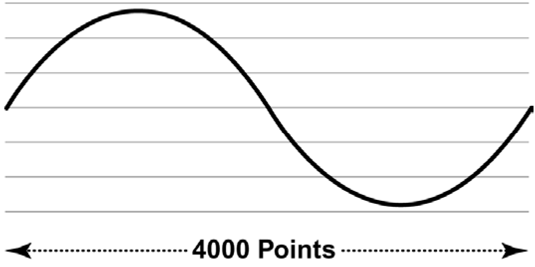
At the stated clock frequency, the samples are about 10 ns apart. This is the time resolution (horizontal) of the waveform. Be sure not to confuse this with the amplitude resolution (vertical).
Carrying this process a step further, assume that the sample RAM contains not one, but four cycles of the waveform:
Foutput = (Clock Frequency ÷ Memory Depth) x (cycles in memory)
Foutput = (100,000,000 ÷ 4000) x (4)
Foutput = (25,000 Hz) x (4)
Foutput = 100,000 Hz
The new frequency is 100 kHz. Figure 23 depicts this concept.
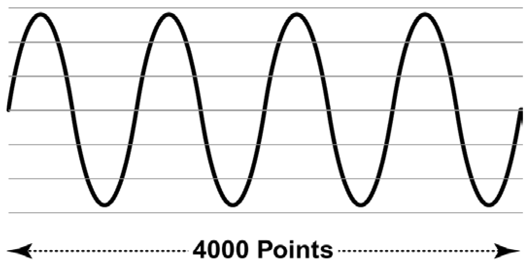
In this instance the time resolution is still 10 ns, but each waveform cycle is represented by only 1000 samples, producing a signal of lower fidelity.
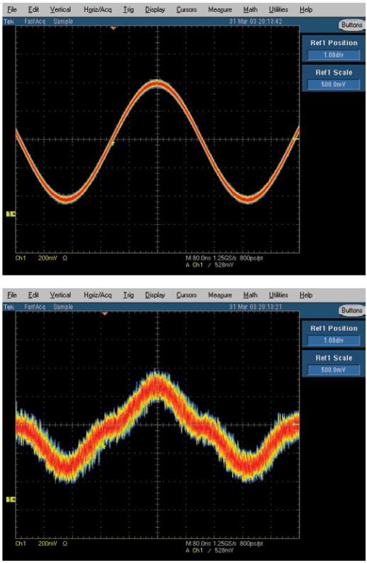
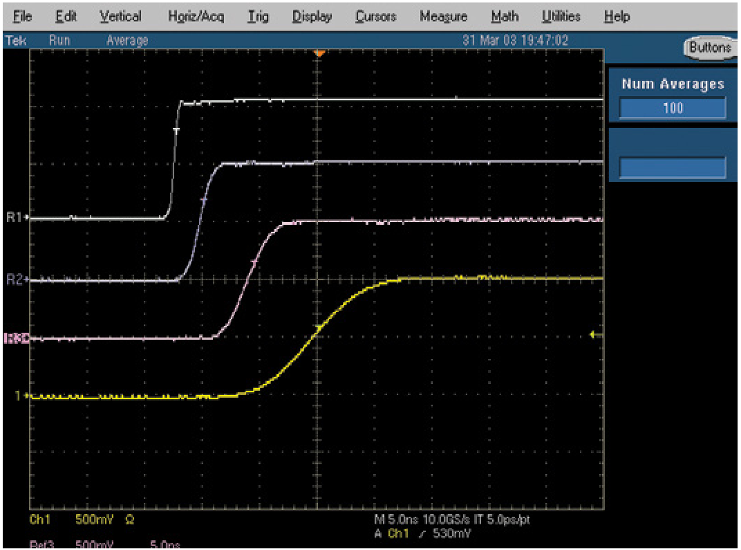
Bandwidth
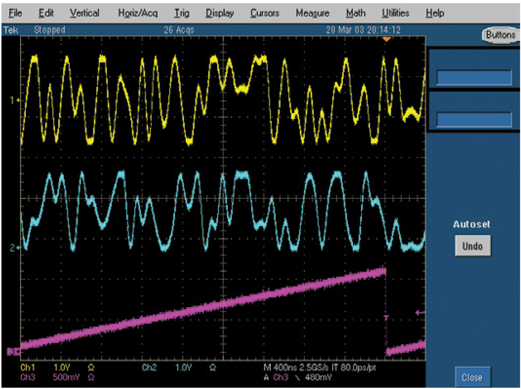
An instrument's bandwidth is an analog term that exists independently of its sample rate. The analog bandwidth of a signal generator's output circuitry must be sufficient to handle the maximum frequency that its sample rate will support. In other words, there must be enough bandwidth to pass the highest frequencies and transition times that can be clocked out of the memory, without degrading the signal characteristics. In Figure 24, an oscilloscope display reveals the importance of adequate bandwidth. The uppermost trace shows the uncompromised rise time of a high-bandwidth source, while the remaining traces depict the degrading effects that result from a lesser output circuit design.
Vertical (Amplitude) Resolution
In the case of mixed signal generators, vertical resolution pertains to the binary word size, in bits, of the instrument's DAC, with more bits equating to higher resolution. The vertical resolution of the DAC defines the amplitude accuracy and distortion of the re-produced waveform. A DAC with inadequate resolution contributes to quantization errors, causing imperfect waveform generation.
While more is better, in the case of AWGs, higher-frequency instruments usually have lower resolution – 8 or 10 bits – than general-purpose instruments offering 12 or 14 bits. An AWG with 10-bit resolution provides 1024 sample levels spread across the full voltage range of the instrument. If, for example, this 10-bit AWG has a total voltage range of 2 Vp-p, each sample represents a step of approximately 2 mV – the smallest increment the instrument could deliver without additional attenuators, assuming it is not constrained by other factors in its architecture, such as output amplifier gain and offset.
Horizontal (Timing) Resolution
Horizontal resolution expresses the smallest time increment that can be used to create waveforms. Typically this figure is simply the result of the calculation:
T = 1/F
where T is the timing resolution in seconds and F is the sampling frequency.
By this definition, the timing resolution of a signal generator whose maximum clock rate is 100 MHz would be 10 nanoseconds. In other words, the features of the output waveform from this mixedsignal generator are defined by a series of steps 10 ns apart.
Some instruments offer tools that significantly extend the effective timing resolution of the output waveform. Although they do not increase the base resolution of the instrument, these tools apply changes to the waveform that reproduce the effect of moving an edge by increments in the picosecond range.
Output Channels
Many applications require more than one output channel from the signal generator. For example, testing an automotive anti-lock brake system requires four stimulus signals (for obvious reasons). Biophysical research applications call for multiple generators to simulate various electrical signals produced by the human body. And complex IQ-modulated telecommunications equipment requires a separate signal for each of the two phases.
In answer to these needs, a variety of AWG output channel configurations has emerged. Some AWGs can deliver up to four independent channels of full-bandwidth analog stimulus signals. Others offer up to two analog outputs, supplemented by up to 16 high-speed digital outputs for mixed-signal testing. This latter class of tools can address a device's analog, data, and address buses with just one integrated instrument.
Digital Outputs
Some AWGs include separate digital outputs. These outputs fall into two categories: marker outputs and parallel data outputs.
Marker outputs provide a binary signal that is synchronous with the main analog output signal of a signal generator. In general, markers allow you to output a pulse (or pulses) synchronized with a specific waveform memory location (sample point). Marker pulses can be used to synchronize the digital portions of a DUT that is at the same time receiving an analog stimulus signal from the mixed-signal generator. Equally important, markers can trigger acquisition instruments on the output side of the DUT. Marker outputs are typically driven from a memory that is independent of the main waveform memory.
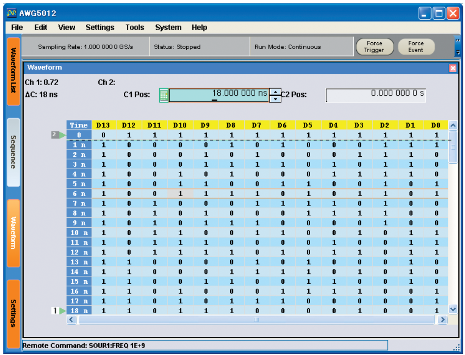
Parallel digital outputs, Figure 29, take digital data from the same memory as the source's main analog output. When a particular waveform sample value is present on the analog output, its digital equivalent is available on the parallel digital output. This digital information is ready-made for use as comparison data when testing digital-to-analog converters, among other things. Alternatively, the digital outputs can be programmed independently of the analog output.
Filtering
Once the basic waveform is defined, other operations, such as filtering and sequencing, can be applied to modify or extend it, respectively. Filtering allows you to remove selected bands of frequency content from the signal. For example, when testing an analog-to-digital converter (ADC), it is necessary to ensure that the analog input signal, which comes from the signal generator, is free of frequencies higher than half the converter's clock frequency. This prevents unwanted aliasing distortion in the DUT output, which would otherwise compromise the test results. Aliasing is the intrusion of distorted conversion by-products into the frequency range of interest. A DUT that is putting out an aliased signal cannot produce meaningful measurements.
One reliable way to eliminate these frequencies is to apply a steep low-pass filter to the waveform, allowing frequencies below a specified point to pass through and drastically attenuating those above the cutoff. Filters can also be used to re-shape waveforms such as square and triangle waves. Sometimes it's simpler to modify an existing waveform in this way than to create a new one. In the past, it was necessary to use a signal generator and an external filter to achieve these results. Fortunately, many of today's high-performance signal generators feature built-in filters that can be controlled.
Sequencing
Often, it is necessary to create long waveform files to fully exercise the DUT. Where portions of the waveforms are repeated, a waveform sequencing function can save you a lot of tedious, memory-intensive waveform programming. Sequencing allows you to store a huge number of "virtual" waveform cycles in the instrument's memory. The waveform sequencer borrows instructions from the computer world: loops, jumps, and so forth. These instructions, which reside in a sequence memory separate from the waveform memory, cause specified segments of the waveform memory to repeat. Programmable repeat counters, branching on external events, and other control mechanisms determine the number of operational cycles and the order in which they occur. With a sequence controller, you can generate waveforms of almost unlimited length.
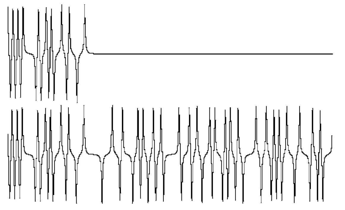
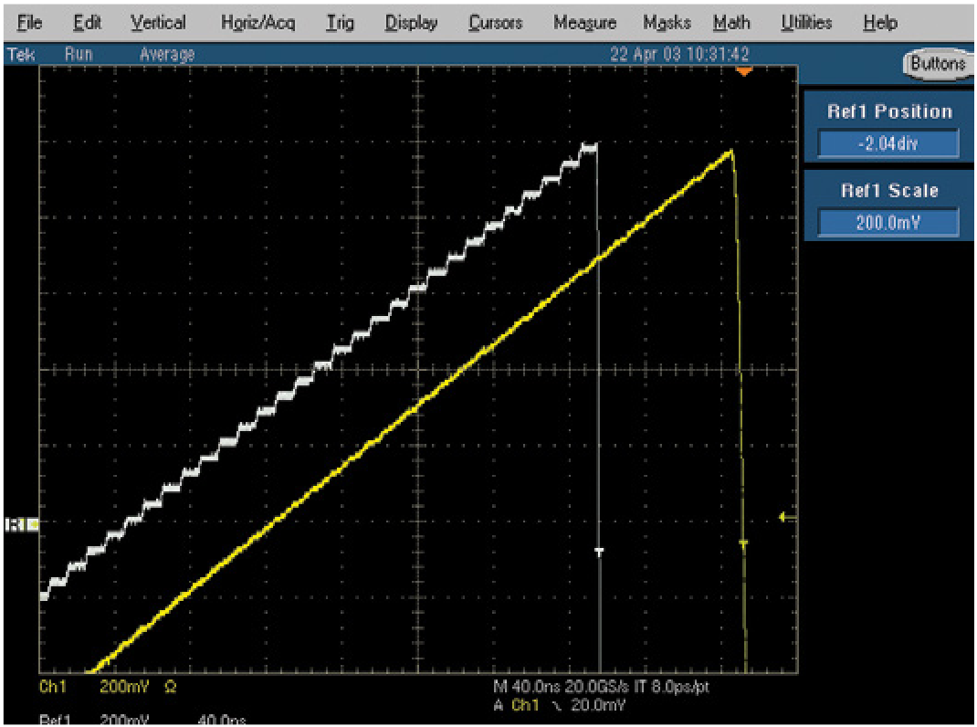
To cite a very simple example, imagine that a 4000-point memory is loaded with a clean pulse that takes up half the memory (2000 points), and a distorted pulse that uses the remaining half. If we were limited to basic repetition of the memory content, the signal generator would always repeat the two pulses, in order, until commanded to stop. But waveform sequencing changes all that.
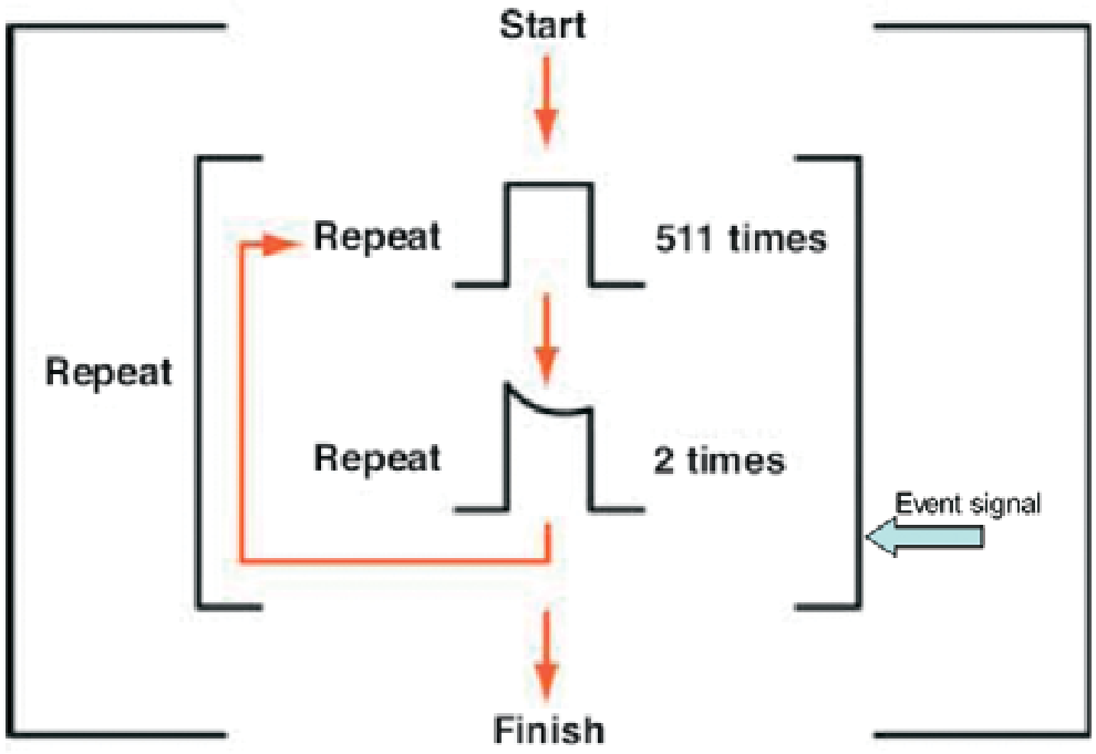
Suppose you wanted the distorted pulse to appear twice in succession after every 511 cycles. You could write a sequence that repeats the clean pulse 511 times, then jumps to the distorted pulse, repeats it twice, and goes back to the beginning to loop through the steps again and again. The concept is shown in Figure 31.
Loop repetitions can be set to infinite, to a designated value, or controlled via an external event input. Considering what we have already discussed about the tradeoff between the number of waveform cycles stored and the resulting timing resolution, sequencing provides much-improved flexibility without compromising the resolution of individual waveforms.
Note here that care must be taken to insure that the phase and magnitude of the sequenced waveform segments transition correctly from the last sample of one segment to the first sample of the next segment. Any flaw in this transition will cause unwanted glitches as the DAC attempts to abruptly change to the new value.
Although this example is very basic, it represents the kind of capability that is needed to detect irregular patterndependent errors. One example is inter-symbol interference in communications circuits. Inter-symbol interference can occur when a signal's state in one cycle influences the signal in the subsequent cycle, distorting it or even changing its value. With waveform sequencing, it is possible to run long-term stress tests – extending to days or even weeks – with the signal generator as a stimulus.
Integrated Editors
Suppose you need a series of waveform segments that have the same shape but different amplitudes as the series proceeds. To create these amplitude variations, you might recalculate the waveform or redraw it using an off-line waveform editor. But both approaches are unnecessarily timeconsuming. A better method is to use an integrated editing tool that can modify the waveform memory in both time and amplitude.
Today's mixed-signal generators offer several types of editing tools to simplify the task of creating waveforms:
- Graphic editor – This tool allows you to construct and view a literal representation of the waveform. The resulting data points are compiled and stored in the waveform memory.
- Sequence editor – This editor contains computer-like programming constructs (jump, loop, etc.) that operate on stored waveforms specified in the sequence.
Data Import Functions
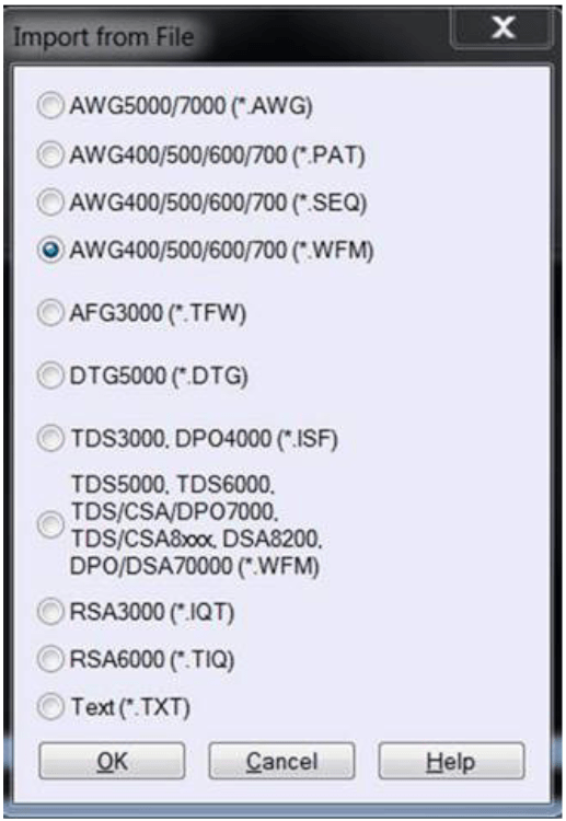
Data import functions allow you to use waveform files created outside the signal generator.
For example, a waveform captured by a modern digital storage oscilloscope can be easily transferred via GPIB or Ethernet to a mixed-signal generator. This operation is key to test methodologies in which a reference signal from a "golden device" is used to test all subsequent production copies of that device. The instrument's editing tools are available to manipulate the signal, just like any other stored waveform.
Simulators and other electronic design automation (EDA) tools are another expedient source of waveforms. With the ability to intake, store, and re-create EDA data, the signal generator can hasten the development of early design prototypes.
The last step in setting up the AWG is to compile files where necessary (as with files from the Equation Editor) and store the compiled files on the hard disk. The "Load" operation brings the waveform into the AWG's dynamic memory, where it is multiplexed and sent to the DAC before being output in its analog form.
These are the basic steps to produce a waveform on an AWG. As explained earlier, waveform files can be concatenated into a sequence using a separate Sequence Editor, yielding a signal stream of almost unlimited length and any degree of complexity.
Creating Complex Waveforms
With today's faster engineering life cycles achieving faster time-to-market, it is important to test designs with realworld signals and characteristics as easily and effectively as possible. In order to generate these real-world signals, they must first be created. Creating these waveforms has historically been a challenge, increasing the time-to-market for the product being designed or tested. With general software tools such as ArbExpress or application specific tools such as SerialExpress® and RFXpress™ creating and editing complex waveforms becomes a much simpler task.
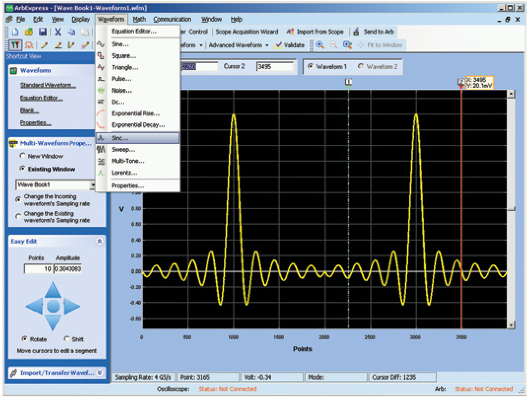
ArbExpress™
ArbExress is a waveform creation and editing tool for AWG and AFG instruments. This Windows-based (PC) application allows capture of waveforms from Tektronix oscilloscopes, or creation from a standard waveform library.
Guided by the Scope Acquisition Wizard, you can conveniently establish a connection to the oscilloscope of choice and select the data source from available channels and memory locations. Waveforms can be imported completely or segments extracted via cursor. Waveforms can also be resampled to match the timing resolution of the destined signal generator.
In ArbExpress, you can also define waveforms freely based on a standard waveform, via point drawing tools or via numerical data table entry. Once you have created a waveform, anomalies can be added easily with math functions or editing tools. Segments or the complete waveform can also be shifted conveniently in time or amplitude axis. This enables real-world signal generation with ease.
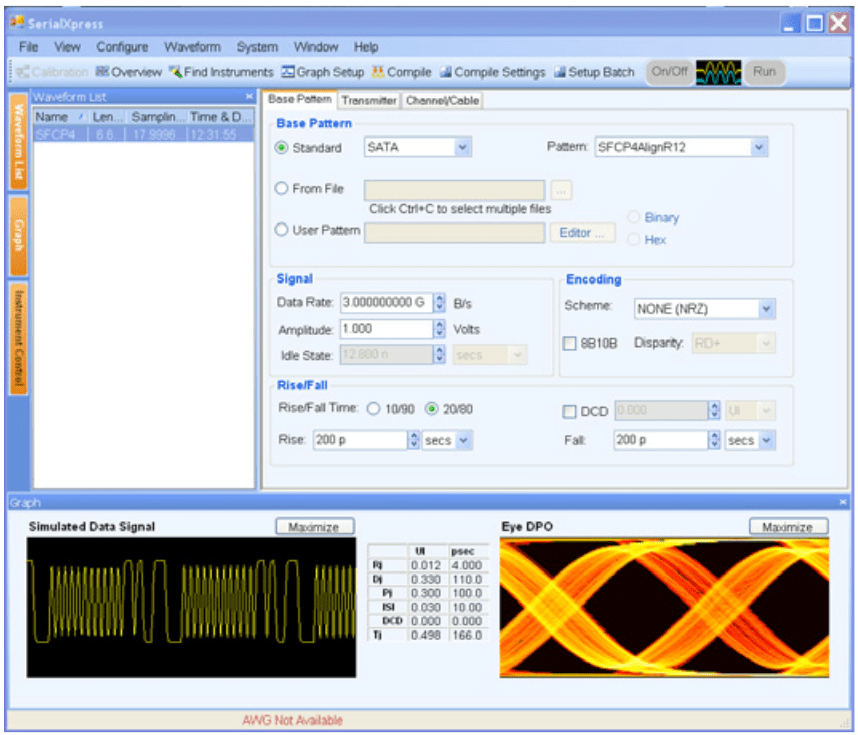
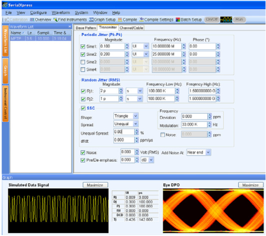
SerialXpress®
The next generation high-speed serial standards can range anywhere from 3 to 6 Gb/s data rates. At these higher speeds new designs are required to operate under diminishing timing margins which mandates the implementation of receiver characterization to compliment conventional transmitter testing. SerialXpress is an application software program that is designed specifically for high speed serial data applications such as SATA, HDMI, PCI-Express, etc. To effectively evaluate circuit behavior and conformance to governing standards, engineers must be able to introduce a variety of known anomalies into the testing process. Periodic jitter, random jitter, pre-emphasis/de-emphasis signals and varying edge rates are just a few of the signal behaviors that must be emulated to insure proper receiver operation.
Application software programs like SerialXpress make it easy for engineers to add signal impairments during conformance testing. In many instances these programs provide the flexibility and signal control that previously required several instruments to attain. Figure 36 & 37 shows the SerialXpress set-up interface for a typical SerialATA (SATA) waveform. Data rates, signal amplitude, rise/fall time and signal impairments can easily be added. SerialXpress also enables users to control the size and magnitude of impairments and each can be analyzed independently or simultaneously with other anomalies.
RFXpress™
RFXpress is a modern PC based software tool with a graphical user interface that allows visual confirmation of waveforms and setups. RFXpress makes waveform synthesis fast and easy with drag and drop waveform editing and Wizard based calibration routines. Enabling users to create the exact waveforms required for extensive, thorough and repeatable design validation for margin and conformance testing. RFXpress considerably cuts the time needed for signal creation and simulations, thus reducing overall development and test time.
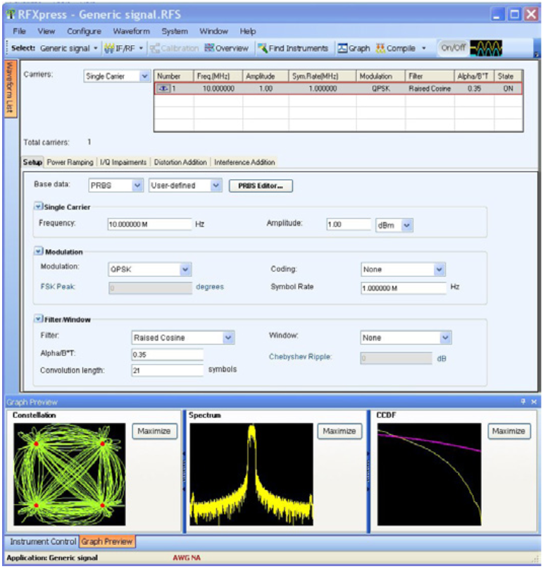
To simplify the waveform creation process for either general purpose or standards based waveforms, RFXpress also incorporates automatic wrap around corrections and normalized waveform amplitude. Automatic wrap around corrections eliminate the spectral glitches that can occur when the waveform is repeated continuously with a large signal amplitude difference between the beginning and end of the waveform.
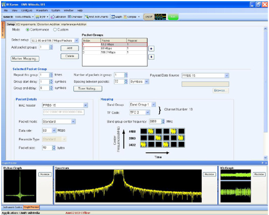
RFXpress provides a special "add-on" option that enables comprehensive WiMedia signal features. For example, though WiMedia defines RF band-groups and center frequencies, engineers may wish to test at IF. RFXpress allows the user to define signals at IF frequencies as well as the standard RF frequencies adopted by WiMedia that are within the AWG's capability.
In the WiMedia conformance mode, complicated MB-OFDM signals can easily be synthesized. RFXpress incorporates adopted WiMedia signal standards, allowing the user to select signal properties at the highest level. This simplifies programming signal features that are dictated by the standard, while reducing the possibility of inadvertent errors when composing signals.
Find the right instrument to power your next project.
Have questions? Get personalized advice for your specific application.
Copyright © Tektronix. All rights reserved. Tektronix products are covered by U.S. and foreign patents, issued and pending. Information in this publication supersedes that in all previously published material. Specification and price change privileges reserved. TEKTRONIX and TEK are registered trademarks of Tektronix, Inc. All other trade names referenced are the service marks, trademarks or registered trademarks of their respective companies.
07.16 76W-16672-7