Introduction
Electronics are continuing to shrink as consumers demand faster, more feature-rich products in ever-smaller form factors. Because of their small sizes, these electronic components usually have limited power handling capability. As a result, when electrically characterizing these components, the test signals need to be kept small to prevent component breakdown or other damage.
Testing these devices and materials often includes making low-voltage measurements. This involves sourcing a known current, measuring the resulting voltage, and calculating resistance. If the device has a low resistance, that resulting voltage will be very small and great care needs to be taken to reduce offset voltage and noise, which can normally be ignored when measuring higher signal levels.
Even if the resistance is far from zero, the voltage to be measured is often very small due to the need to source only a small current in order to avoid damaging the device. This power limitation often makes characterizing the resistance of modern devices and materials very challenging.
This article discusses techniques to eliminate thermoelectric voltages to allow more accurate resistance measurements, including a three-step delta measurement method for low-power/low-voltage applications. In addition, it also presents a method for accurately making differential conductance measurements.
Low-Level Voltage Measurements
There are many factors that make low voltage measurements difficult. For instance, various noise sources can hinder resolving the actual voltage, and thermoelectric voltages (thermoelectric EMFs) can cause error offsets and drift in voltage readings. In the past, it would have been possible to simply increase the test current until the DUT’s response voltage was much larger than these errors, but with today’s smaller devices this is no longer an option. Increased test current can cause device heating, changing the device’s resistance, or even destroy the device. The key to obtaining accurate, consistent measurements is eliminating the error. For low-voltage measurement applications, such error is composed largely of white noise (random noise across all frequencies) and 1/f noise. Thermoelectric voltages (typically having 1/f distribution) are generated from temperature differences in the circuit.
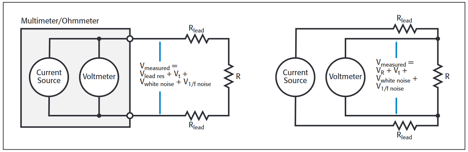
Resistance is calculated using Ohm’s Law; that is, the DC voltage measured across the device divided by the DC stimulus current yields the resistance. The voltage readings will be a sum of the induced voltage across the device (VR), lead and contact resistance (Vlead res), other 1/f noise contributions (V1/f noise), and white noise (Vwhite noise), and thermoelectric voltages (Vt). Using four separate leads to connect the voltmeter and current source to the device eliminates lead resistance, because the voltmeter won’t measure the voltage drop across the source leads. Implementing filtering may reduce white noise but will not reduce 1/f noise significantly, which often sets the measurement noise floor.
Thermoelectric voltages normally have a 1/f characteristic. This means there can be significant offset, and the more measurements that are made the more drift. Taken together, the offset and drift may even exceed VR, the voltage across the DUT induced by the applied current. It’s possible to reduce thermoelectric voltages using techniques such as all-copper circuit construction, thermal isolation, precise temperature control, and frequent contact cleaning.
No matter what steps are taken to minimize thermoelectric voltages, it’s impossible to eliminate them. It would be preferable to have a method that would allow accurate resistance measurements even in the presence of large thermoelectric voltages, instead of working to minimize them.
The Delta Method of Measuring Resistance
One way to eliminate a constant thermoelectric voltage is to use a delta method wherein voltage measurements are made first at a positive then at a negative test current. A modified technique can be used to compensate for changing thermoelectric voltages. Over the short term, thermoelectric drift can be approximated as a linear function. The difference between consecutive voltage readings is the slope or the rate of change in thermoelectric voltage. This slope is constant, so it may be canceled by alternating the current source three times to make two delta measurements – one at a negativegoing step and one at a positive-going step. For the linear approximation to be valid, the current source must alternate quickly and the voltmeter must make accurate voltage measurements within a short time interval. If these conditions are met, the three-step delta technique yields an accurate voltage reading of the intended signal unaffected by thermoelectric offsets and drifts.
An analysis of the mathematics for one three-step delta cycle will demonstrate how the technique compensates for temperature differences in the circuit, thereby reducing measurement error. Consider the example in Figure 2a :
Test current = ±5nA ;
Device = 500Ω resistance
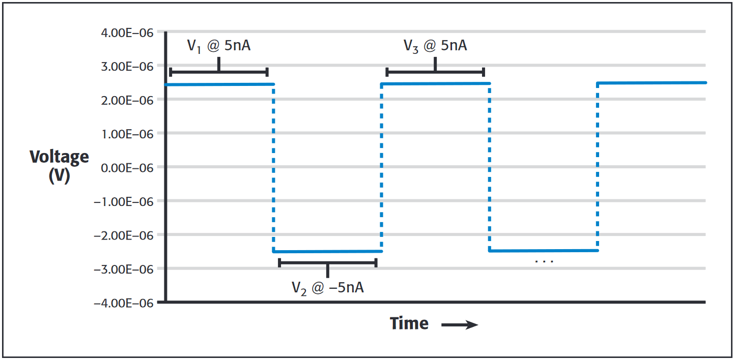
Ignoring thermoelectric voltage errors, the voltages measured at each of the steps are:
V1 = 2.5µV ; V2 = –2.5µV ; V3 = 2.5µV
Let's assume the temperature is linearly increasing over the short term in such a way that it produces a voltage profile like that shown in Figure 2b, where Vt is climbing 100nV with each successive reading.
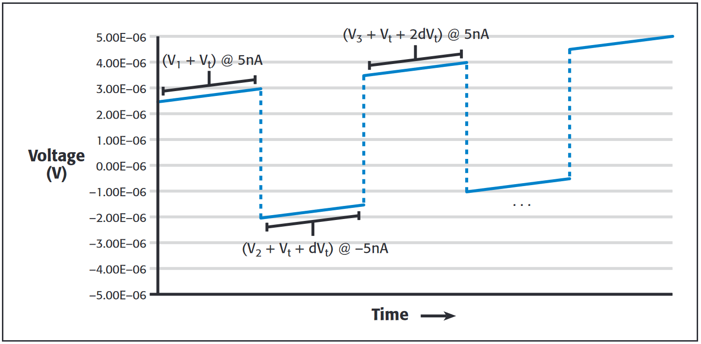
As Figure 2b shows, the voltages now measured by the voltmeter include error due to the increasing thermoelectric voltage in the circuit and are no longer of equal magnitude. However, the absolute difference between the measurements is in error by a constant 100nV, so it’s possible to cancel this term. The first step is to calculate the delta voltages. The first delta voltage (Va) is equal to:
Va = negative-going step = (V1 – V2)/2 = 2.45 µV
The second delta voltage (Vb) is made at the positive-going current step and is equal to:
Vb = positive-going step = (V3 – V2)/2 = 2.55 µV
The thermoelectric voltage adds a negative error term in Va and a positive error term in the calculation of Vb. When the thermal drift is linear, these error terms are equal in magnitude. Thus, we can cancel the error by taking the average of Va and Vb :
Vf = final voltage reading = (Va + Vb)/2 = ½[(V1 – V2)/2 + (V3 – V2)/2] = 2.5 µV
The delta technique eliminates error due to changing thermoelectric voltages
Therefore, the voltmeter measurement is the voltage induced by the stimulus current alone. As alternation continues, every successive reading is the average of the three most recent A/D conversions.
The three-step delta technique is the best choice for high-accuracy resistance measurements. Figure 3 compares 1,000 measurements of a 100Ω resistor made with a 10nA test current taken over approximately 100 seconds. In this example, the rate of change in thermoelectric voltage is no more than 7µV/s. The two-step delta technique fluctuates 30% as the thermoelectric error voltage drifts. In contrast, the three-step delta technique has much lower noise—the measurement is unaffected by the thermoelectric variations in the test circuit.
Equipment Requirements
The success of the three-step delta method depends on the linear approximation of the thermal drift viewed over a short time interval. This approximation requires that the measurement cycle time be faster than the thermal time constant of the test system. This imposes certain requirements on the current source and voltmeter used.
The current source must alternate quickly in evenly timed intervals so the thermoelectric voltage changes an equal amount between each measurement.
The voltmeter must be tightly synchronized with the current source and capable of making accurate measurements in a short time interval. Synchronization favors hardware handshaking between the instruments so that the voltmeter can make voltage measurements only after the current source has settled and the current source doesn’t switch polarity until after the voltage measurement has been completed. The measurement speed of the voltmeter is critical in determining total cycle time; faster voltage measurements mean shorter cycle times. For reliable resistance measurements, the voltmeter must maintain this speed without sacrificing lownoise characteristics.
In low-power applications, the current source must be capable of outputting low values of current so as not to exceed the maximum power rating of the device. This ability is particularly important for moderately high- and high-impedance devices.
Differential Conductance
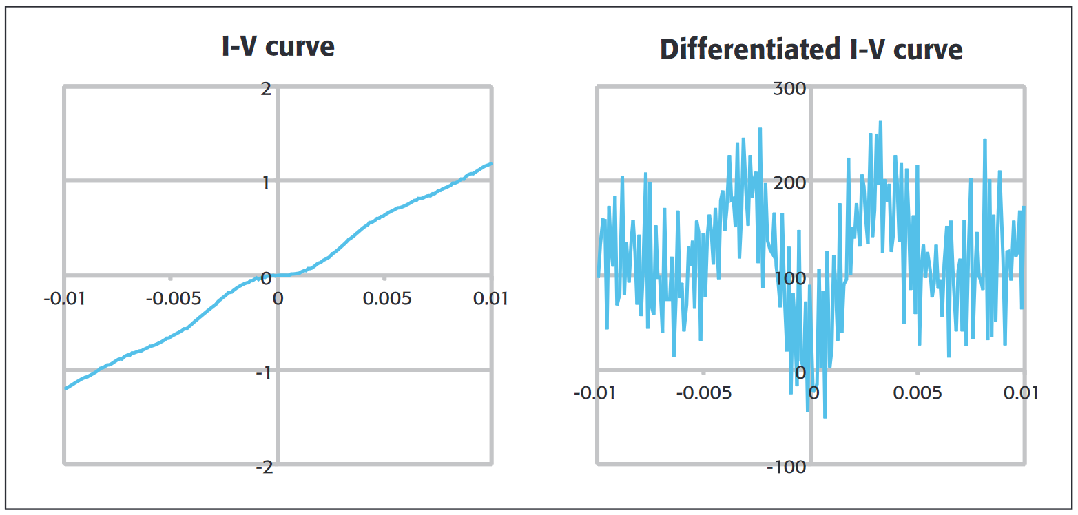
Another important measurement technique for characterizing solid-state and nanoscale devices is differential conductance. For these materials, things are rarely simplified to Ohm’s Law. With these nonlinear devices, the resistance is no longer a constant, so a detailed measurement of the slope of that I-V curve at every point is needed to study them.This derivative is called the differential conductance, dG = dI/dV (or its inverse, the differential resistance, dR = dV/dI). The fundamental reason that differential conductance is interesting is that the conductance reaches a maximum at voltages (or more precisely, at electron energies, in eV) at which the electrons are most active. In different fields, this measurement may be called electron energy spectroscopy, tunneling spectroscopy, or density of states.
Typically, researchers perform differential conductance measurements using one of two methods: obtaining an I-V curve with a calculated derivative or using an AC technique. The I-V curve method requires only one source and one measurement instrument, which makes it relatively easy to coordinate and control. A current-voltage sweep is made and the mathematical derivative is found. However, taking the mathematical derivative amplifies any measurement noise, so tests must be run multiple times and the results averaged to smooth the curve before the derivative is calculated. This leads to long test times.
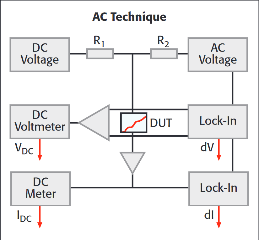
The AC technique reduces noise and test times. It superimposes a low amplitude AC sine wave on a swept DC bias. This involves many pieces of equipment and is hard to control and coordinate. Assembling such a system is time consuming and requires extensive knowledge of electrical circuitry. So while the AC technique produces marginally lower noise, it is much more complex.
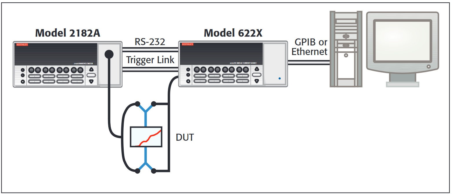
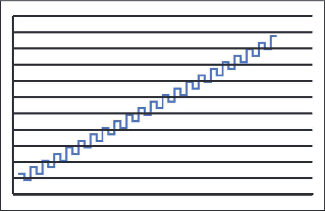
There is, however, another way to obtain differential conductance measurements that is both simple and low noise. This technique involves a current source that combines the DC and AC components into one instrument. There is no need to do a secondary measure of the current, because the instrument is a true current source. Figure 7 shows the current sourced in a differential conductance measurement. The waveform can be broken down into an alternating current and a staircase current. Using the exact same calculations as in the delta method, accurate resistance or conductance measurements can be made, with measurements at each point of the staircase. Because the three-step delta technique eliminates linearly drifting offsets, it is also immune to the effects of our linearly changing staircase. In addition, the nanovoltmeter used in this method has lower noise than lock-in amplifiers at the alternation frequency.
There are several benefits to this method. One is that in the areas of highest conductance, more data points are taken by sourcing the sweep in equal current steps. These areas are of most interest to researchers and give detailed data. In addition, having just one instrument that both sources current and measures voltage greatly simplifies equipment setup. Lastly, the reduced noise can lower test times from an hour to only five minutes
Conclusion
Thermoelectric EMFs are often the dominant source of error in low resistance/low power resistance measurements. This error may be almost completely removed using a three-point current reversal technique. Using this new technique means it’s no longer necessary to take extreme care to minimize thermally induced voltage noise in the wiring of resistance measuring systems, greatly simplifying the measurement process. Applying the same technique to differential conductance measurements greatly reduces noise and test complexity.
Find more valuable resources at TEK.COM
Copyright © Tektronix. All rights reserved. Tektronix products are covered by U.S. and foreign patents, issued and pending. Information in this publication supersedes that in all previously published material. Specification and price change privileges reserved. TEKTRONIX and TEK are registered trademarks of Tektronix, Inc. All other trade names referenced are the service marks, trademarks or registered trademarks of their respective companies.
No.2636 1005