High impedance insulators are an integral part of today's high performance electronic products. The purity of the materials used to construct these insulators can make the difference between a product that works properly and one that doesn't work at all. The accepted method of measuring high resistance is to apply a large voltage to a sample and measure the small currents stimulated through that sample. However, for high resistance samples, the levels of current that must be measured are extremely low, so testing these materials accurately and repeatably can be a challenge. Other current sources,such as piezoelectric effects or discharging capacitive elements, can obscure the stimulated current one wishes to observe in order to calculate resistance and surface and volume resistivity. This paper presents a method for selectively measuring a stimulated current in the presence of other currents that may be five to ten times the magnitude of the stimulated current.
While resistance and resistivity are related properties, they are not synonymous. Resistivity is a property of the material itself, so it's independent of the geometry of a particular sample. In contrast, resistance depends not only on the material but on the length and cross-sectional area of the sample being measured. When making volume resistivity measurements, the measured resistance is multiplied by the cross-sectional area of the sample perpendicular to the current flow, then that value is divided by the path length of the current.The results are typically expressed in Ω-cm. When working with samples with complex geometries, effective area and thickness values are used in the calculation. For surface resistivity measurements, the measured resistance is multiplied by the width of the surface across which the current flows, then that value is divided by the path length of the current along the surface. Results are expressed in Ω/. If the electrodes in the text fixture or the sample have complex geometries,effective multiplier values are used in the calculation.
A resistivity test system usually consists of a picoammeter, voltage source, and a specialized test fixture with electrodes for making electrical contact with the sample. Standard fixture parameters and dimensions have been defined by the American Society for Testing and Materials (ASTM) for measuring volume and surface resistivity and are commercially available. Figure 1 is a cutaway drawing of a fixture based on the ASTM D257 standard.

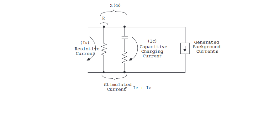
The standard way to characterize high-resistance (low conductance) samples is to apply a step voltage, measure the current through the sample after a fixed time, then calculate the resistance in accordance with Ohm’s Law (R=V/I). However, it's important to understand that the current measured this way is a combination of background currents from many sources, the DC resistive current, and the current charging the capacitance of the material.(See Figure 2.) Any sample has capacitance, as well as resistance. In fact, any sample can best be modeled as a collection of resistances ("R"s) and capacitances ("C"s). Circuit modeling of materials has been covered extensively in the literature.
When designing an experiment, it's important to consider the characteristic frequency at which the sample is to be measured. A one-minute delay between the step voltage and the measurement is effectively a measurement of the material’s 8.3mHz response. In many cases, this is perfectly adequate. In fact, a 15 second wait (33mHz) will often give a good approximation of DC response. At any rate, the user should make the measurement at a frequency that ensures the result is relevant to the sample's fitness-for-use. Once the characteristic frequency has been selected, it's essential to make an accurate and repeatable measurement of the response at that frequency. While one may or may not wish to include the low-frequency AC impedance in the sample measurement, the background currents are not an effect of the applied voltage and have no relevance in any impedance measurement.
The measurement technique that follows uses alternating DC voltages to eliminate the effects of these background currents and drifts.
Before any measurement can be considered valid, the accuracy of the measurement instrumentation and fixturing must be checked. A good way to do this is to measure a sample of air using the same technique as that used when measuring samples. To do this, simply insert a spacer between the ring electrode (guard ring) and top electrode of a standardized fixture to separate the picoammeter input electrode from the other two electrodes.
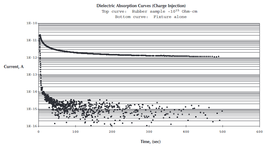
Figure 3 shows leakage currents in response to a step voltage in the test setup used for this experiment. The sample currents are from a 1015W-cm sample of rubber. In this case, the fixture leakage currents are lower than the sample currents by a factor of 1000. Without further modifications, this system will measure resistances an order of magnitude higher than that, without substantially shunting the sample.
Background currents can be produced by many different phenomena, from piezoelectric effects to temperature induced pole relaxation to discharging internal capacitive elements. These background currents decay over time at different rates, depending upon their individual time constants. Figure 4 shows a typical background current and a step response current superimposed on it. The standard method current is the sum of the step response stimulated current and the background current.
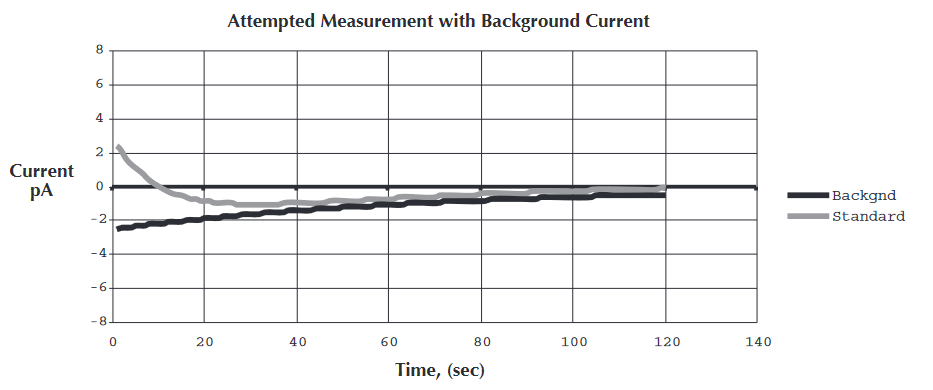
As Figure 4 indicates, the stimulated current is completely masked by the background current. This would lead to the erroneous conclusion that the sample has negative resistance. This has very interesting implications for reciprocal measurements, such as resistance. The resistance "measurement" is really a calculated value from a known voltage divided by a measured current; therefore, the uncertainty of the result may increase radically. For example, a voltage measurement with a signal-to-noise ratio of >1 can be improved by averaging. However, the accuracy of a resistance measurement that has an underlying current measurement with a signal-to-noise ratio of <1 cannot be improved by averaging. When the value of the signal plus the offset ("noise") passes through zero, the calculated resistance shoots to negative infinity (-∞) by way of positive infinity (+∞). No amount of averaging will cure the problems that result from high noise in a reciprocal type measurement because these calculations literally have ±∞ uncertainty. This is sometimes jokingly referred to as "noise in the exponent."
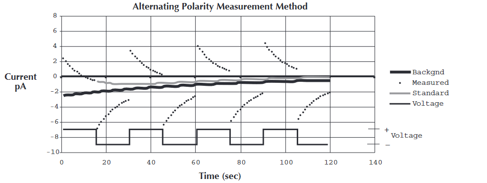
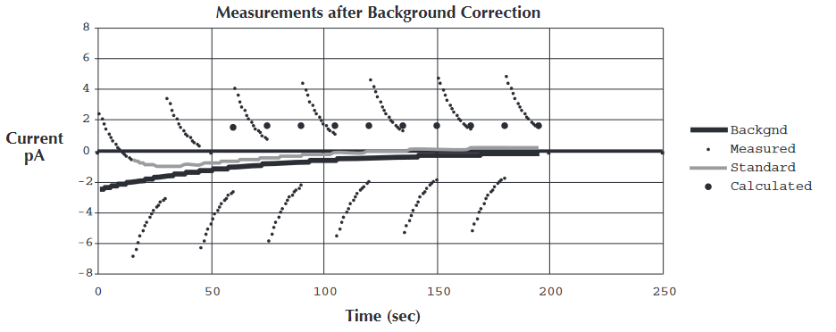
In contrast, Figure 5 shows the sample's current response to step voltages of alternating polarity superimposed on the background current.
The actual measurement procedure is to:
- Apply a positive voltage, wait for the specified period (chosen as 15 seconds above), then take a current measurement.
- Immediately afterwards, apply a negative voltage of the same magnitude. After waiting the specified time, take another current measurement
Figure 5 illustrates the sample current with the measured points shown as solid squares at the ends of each current tail. These points were measured just before the voltage was reversed. The first two measurements essentially make it possible to perform a ∆V/∆I calculation. To cancel out first order drift of the background, repeat step 1. Repeating step 2 o get a fourth measurement point with a negative voltage will cancel out second order drift (curvature), which is usually sufficient for the level of accuracy required. These cancellations are easily done as averages weighted with the binomial coefficients of that order. For example, a measurement of I1, I2, and I3, (where I2 is the negative polarity measurement) is used as follows: Icalc = (I1+2(-I2)+I3)/4. Icalc is the current superimposed on the background current in response to the stimulus voltage, so Z = ∆V/∆I = V0/Icalc. Calculated current for second order correction is:
(I1+3(-I2)+3(I3)+(-I4))/8.
In Figure 6 the resulting calculated currents are shown as "X"s. The values of the first four measured currents are -0.552, -3.094, 0.301, and -2.677 pA respectively
Note that not all of these currents are of the polarity that might be expected, given the polarity of the voltages applied (+, –, +, –).
The current calculation would be performed thus:
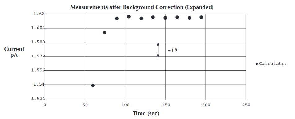
| Icalc = | (+)(–0.552) + (–)3(–3.094) + (+)3(0.301) + (–)(–2.677) | = 1.539pA |
| 8 |
The alternating positive and negative signs used for the terms are the polarities of the voltages used to generate the respective currents (I1, I2…) The voltage used was ±50V, so the impedance is 50V/1.539×10-12A = 3.249×10¹³Ω. Factoring in an area of 21.44 cm2 (effective area of the guarded electrode) and a sample thickness of 0.18 cm yields 3.870×10¹⁵Ω-cm.
It is clear by examining the calculated points (the "•"s), that this technique provides much more repeatable results than measuring current directly (the smaller dots). Figure 7 shows an expanded view of the calculated current values. The sequence of weighted averages quickly converges to a very stable value. An RC circuit takes a finite amount of time to respond to an AC stimulus, so the first few currents measured are not yet steady state values with respect to the low frequency alternating voltage. The magnitude of this error at a given step number is primarily dependent on the magnitude and time constant of the background current. In practice, with background currents that are less than five times the stimulated current, the third current value is within 1% of steady state. For the data presented here, the first two measurements are ignored for the purpose of the calculation, and the next four are used to cancel out the second order background currents and give the stimulated current to within 0.3% of the steady state value.
Measurement timing is extremely critical. At each measurement point, the decaying current of a charging RC circuit is being measured. Thus, if a single measurement point is given a longer time to decay, the measured current will be less than the rest. If all stimulated currents are to be within 0.1% of each other, the timing jitter must be less than 0.001τ, where τ is the dominant time constant of the sample. That is, -∆t/τ = ln(0.999) = -0.001. For example, the sample in Figure 3 has a dominant time constant of 17sec at the measurement point. Therefore, to ensure less than 0.1% error due to timing, this would require that subsequent measurements have less than 17msec of timing jitter.
Experimental results
In our experiments, we studied three basic types of samples: rubber, clear rigid vinyl plastic, and epoxy. The epoxy sample was a piece of standard FR4 printed circuit board substrate. With the standard R=V/I test method, the epoxy’s volume resistivity was measured to be anywhere from 1014 Ω-cm up to 1018 Ω-cm and from -1018Ω-cm to -1015Ω-cm. A user would not be able to use these results, except to speculate that the actual resistivity is above 1014Ω-cm. Although the resistivity was not extremely high, the random background currents generated were sufficient to offset the readings significantly. Using the methods detailed in this paper, the resistivity values were measured at 3.80 × 10¹⁴ Ω-cm, repeatable to 3% p-p, as shown in Figure 8.

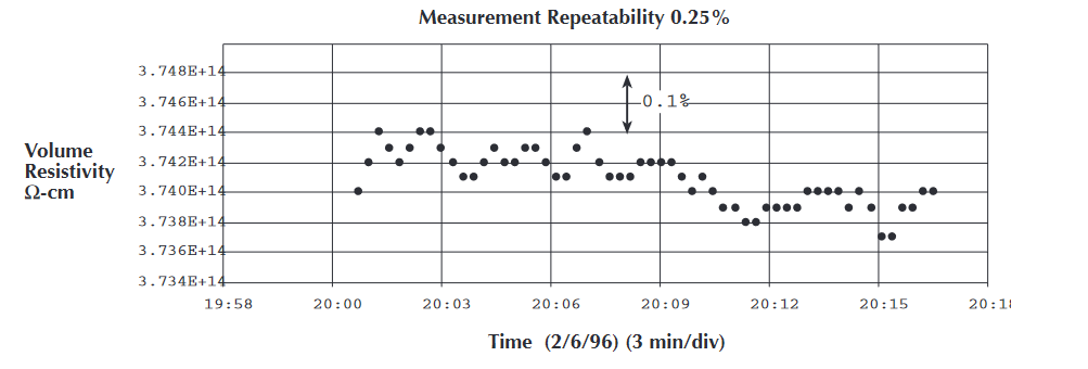
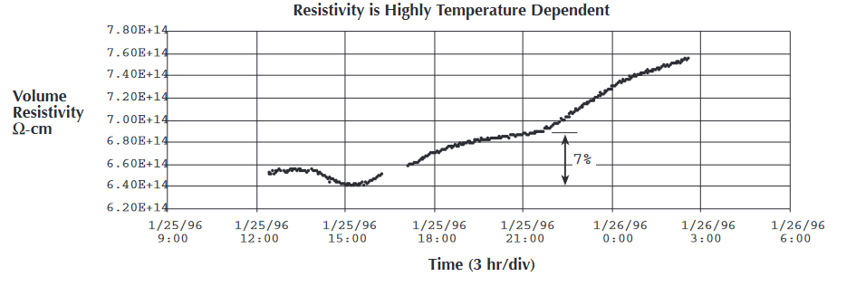
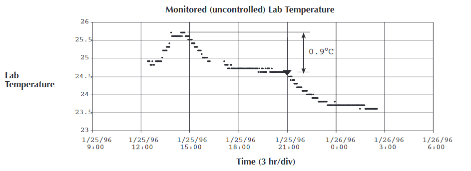
If the view of a single measurement run is expanded (Figure 9), it shows that the measurement itself is stable to within 0.3% p-p, but the material itself has an extremely high resistivity temperature coefficient. A temperature change of just 1°C resulted in a 3% change in the material's resistivity. Locating the sample in an environment controlled to within ±1°C improved measurement repeatability to 2.5% p-p. However, even in a ±1°C environment, each time the test fixture was opened, the temperature of the sample changed sharply, and it required several hours for the resistance to resettle near the original value. This increased measurement variations to about 3% p-p.
If the instrumentation allows monitoring temperature, it is possible to measure the temperature coefficient of the material's resistance. As shown in Figures 10a and 10b, the resistivity of a vinyl sample was measured while the ambient temperature was monitored. The sample exhibited a very clear correlation between increasing temperature and decreasing resistivity. In fact, the Tc could be pinned down to (8% ± 1%)/°C. The short term repeatability was on the order of 0.2% p-p, indicating that the instrumentation was not the limiting factor in the accuracy of the measurement in this setup.
The Alternating Polarity method can also improve the reproducibility of surface resistivity measurement results. Using the same FR4 material and the same measurement technique, we were able to measure the material's surface resistivity of 1.36 × 10¹⁵Ω/ with p-p deviations of less than 7% with only ±1°C control over the ambient temperature. In contrast, the standard method yielded values widely scattered, between 1013Ω/ and 1018Ω/ and between -1013Ω/ and -1018Ω/ . Only half the readings were even positive.
With the rubber sample, the standard test method yielded results of 1014-1015Ω-cm, with frequent negative readings. The value might be guessed at within two orders of magnitude. The new algorithm provided results that varied by less than 4%, and that variation was attributed to temperature variations. This material has a resistivity temperature coefficient of 5%/°C (50,000ppm/°C), making the inability to control the temperature with extreme precision the limiting factor in this measurement.
Similarly, with the vinyl sample, the standard test method yielded results of anywhere from 1014-1016Ω-cm and many of the readings were negative. The new algorithm provided results of 6.8 × 10¹⁴Ω-cm, which varied by less than 7% due to temperature variations.
High resistivity measurements are particularly sensitive to the extraneous background currents that plague any low current measurement. The Alternating Polarity method presented here makes it possible to measure high resistivities with precision without waiting hours in the hopes that background currents will decay to a sufficiently low level. This method allows the measurement of extremely high resistivities with a repeatability of a few percent, even in the presence of background currents that would otherwise lead to literally infinite error.
Find more valuable resources at TEK.COM
Copyright © Tektronix. All rights reserved. Tektronix products are covered by U.S. and foreign patents, issued and pending. Information in this publication supersedes that in all previously published material. Specification and price change privileges reserved. TEKTRONIX and TEK are registered trademarks of Tektronix, Inc. All other trade names referenced are the service marks, trademarks or registered trademarks of their respective companies.
No.1808 6013KIKN22w