THIS APPLICATION NOTE
- Is designed help product designers or EMC engineers learn the basics of EMC and EMI troubleshooting and debug
- Introduces a 3-step process for EMI Troubleshooting
- Gives an overview of Radiated and Conducted Emissions Troubleshooting, including tips for setups
- Explains how to interpret measurement data
- Describes techniques for dealing with ambient RF during testing
- Gives several detailed troubleshooting examples using time-correlated waveforms and spectrums
The app note explains specifically how to use 4/5/6 Series MSOs with built-in digital downconverters and Spectrum View. This patented technology enables you to simultaneously view both analog and spectral views of all your analog signals, with independent controls in each domain. Spectrum View makes oscilloscope-based frequency-domain analysis as easy as using a spectrum analyzer while retaining the ability to correlate frequencydomain activity with other time-domain phenomena.
Electromagnetic compatibility (EMC) and the related electromagnetic interference (EMI) must be addressed prior to marketing commercial or consumer electronic products, as well as military and aerospace equipment. EMC or EMI compliance is often left to the end of a project and last-minute failures often result in schedule delays, unplanned cost and stress on the engineering team. Having the right tools and techniques available can help head off problems and address them quickly when they occur.
Briefly, radiated emissions is a measure of the radiated E-fields, while conducted emissions is a measure of the conducted EMI currents emanating from the product, equipment, or system under test. There are worldwide limits on how high these emissions can be, depending on the environment in which the equipment is designed to work.
Today, with the myriad of consumer electronic products, including wireless and mobile devices, compatibility between devices is becoming even more important. Products must not interfere with one another (radiated or conducted emissions) and they must be designed to be immune to external energy sources. Most countries now impose some sort of EMC standards to which products must be tested.
Basic Definitions
Let’s start with some basic definitions, and there’s a subtle difference between EMC and EMI.
- EMC implies that the equipment being developed is compatible within the expected operating environment. For example, a ruggedized satellite communications system when mounted in a military vehicle must work as expected, even in the vicinity of other high-powered transmitters or radars. This implies both emissions and immunity compatibility in close environments. This usually applies to military and aerospace products and systems, as well as automotive environments. Radiated emissions is usually measured at a 1m test distance.
- EMI (also sometimes referred to as radio frequency interference, or RFI) is more concerned with a product interfering with existing radio, television, or other communications systems, such as mobile telephone. Outside the U.S. it also includes immunity to external energy sources, such as electrostatic discharge and power line transients. This usually applies to commercial, consumer, industrial, medical, and scientific products. Radiated emissions is usually measured at a 3 m or 10 m test distance. This app note will focus on EMI Troubleshooting.
EMI Troubleshooting
A THREE-STEP PROCESS FOR EMI TROUBLESHOOTING
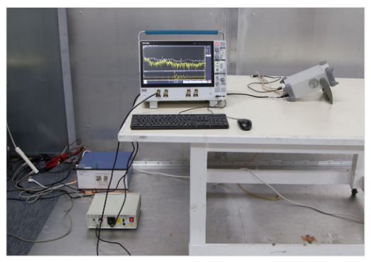
Many product designers may be familiar with how near field probes may be used to identify EMI “hot spots” on PC boards and cables but may not know what to do next with this information. We’ll use Tektronix Spectrum View on a 6 Series Mixed Signal Oscilloscope as an example. Here’s a simple three-step process for EMI troubleshooting.
Step 1 - Use near field probes (either H- or E-field) to identify energy sources and characteristic emission profiles on the PC board and internal cables. Energy sources generally include clock oscillators, processors, RAM, D/A or A/D converters, DC-DC converters, and other sources, which produce high frequency, fast-edged, digital signals. If the product includes a shielded enclosure, probe for leaky seams of other apertures. Record the emission profile of each energy sources.
Step 2 - Use a current probe to measure high frequency cable currents. Remember, cables are the most likely structure to radiate RF energy. Move the probe back and forth along the cable to maximize the highest harmonic currents. Record the emission profile of each cable.
Step 3 - Use a nearby antenna (typically, a 1 m test distance) to determine which of the harmonic signals actually radiate. Record these harmonics and compare to the near field and current probe cable measurements. This will help you determine the most likely energy sources that are coupling to cables or seams and radiating to the antenna.
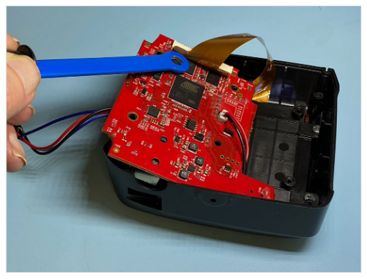
STEP 1 - Near Field Probing- Most near field probe kits come with both E-field and H-field probes. Deciding on H-field or E-field probes depends on whether you’ll be probing currents – that is, high di/dt – (circuit traces, cables, etc.) or voltages – that is, dV/dt – (switching power supplies, etc.) respectively. Most troubleshooting is done with H-field probes, because we’re usually interested in tracing high frequency harmonic currents. The smaller diameter ones provide higher resolution but may need preamplification to boost their signals. However, both H- and E-field probes are useful for locating leaky seams or gaps in shielded enclosures.
Start with the larger H-field probe and sniff around the product enclosure, circuit board(s), and attached cables. The objective is to identify major EMI sources and dominant narrow band and broadband frequencies. Document the locations and frequency characteristics observed. As you zero in on sources, you may wish to switch to the middlesized (1 cm) H-field probe (Figure 1), which will offer greater resolution (but slightly less sensitivity). You may find most probing is eventually done with this probe.
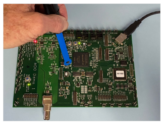
Also, note that H-field probes are most sensitive (will couple the most magnetic flux) when their plane is oriented in parallel with the trace or cable. It’s also best to position the probe at 90 degrees to the plane of the PC board. See Figure 2.
Remember that not all sources of high frequency energy located on the board will actually radiate! Radiation requires some form of coupling to an “antenna-like” structure, such as an I/O cable, power cable, or seam in the shielded enclosure.
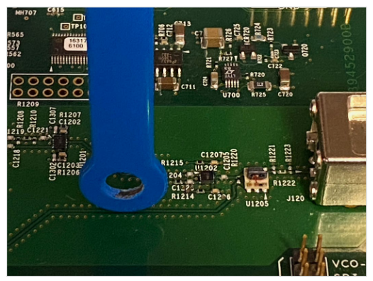
When applying potential fixes at the board level, be sure to tape down the near field probe to reduce the variation you’ll experience in physical location of the probe tip. Remember, we’re mainly interested in relative changes as we apply fixes.
STEP 2 - Current Probe Measurements- Next, measure the attached common mode cable currents (including power cables) with a high frequency current probe, such as the Com-Power CLCE-400, or equivalent (Figure 3). Document the locations of the top several harmonics and compare with the list determined by near field probing. These will be the most likely to radiate and cause test failures because they are flowing on antenna-like structures (cables).
Note that it only takes only 5 to 8 μA of high frequency current to fail the FCC or CISPR Class B test limits. Using the manufacturer’s supplied transfer impedance calibration curve will help you calculate the current from the analyzer voltage at the probe port.
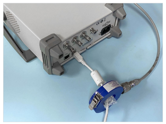
It’s a good idea to slide the current probe back and forth to maximize the harmonics. This is because some frequencies will resonate in different places, due to standing waves on the cable.
It’s also possible to predict the radiated E-field (V/m) given the current flowing in a wire or cable, with the assumption the length is electrically short at the frequency of concern. This has been shown to be accurate for 1m long cables at up to 200 MHz. Refer to Reference 1, 2, or 5 for details.
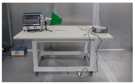
STEP 3 - Troubleshooting with a Close-Spaced Antenna - Once the product’s harmonic profile is fully characterized, it’s time to see which harmonics actually radiate. To do this, we can use an uncalibrated antenna connected to a 4/5/6 Series MSO spaced at least 1m away from the product or system under test to measure the actual emissions (Figure 4). Typically, it will be radiation from attached I/O or power cables, as well as leakage in seams or apertures of the shielded enclosure. Compare this data to that of the near field and current probes. The actual measured emissions should indicate the energy source as identified by the previous probing.
Try to determine if cable radiation is the dominant issue by removing the cables one by one. You can also try installing a ferrite choke on one, or more, cables as a test. Use the near field probes to determine if leakage is also occurring from seams or openings in the shielded enclosure.
Once the emission sources are identified, you can use your knowledge of filtering, grounding, and shielding to mitigate the problem emissions. Try to determine the coupling path from inside the product to any outside cables. In some cases, the circuit board may need to be redesigned by optimizing the layer stack-up or by eliminating high speed traces crossing gaps in return planes, etc. By observing the results in real time with an antenna spaced some distance away, the mitigation phase should go quickly
Radiated and Conducted Emissions Troubleshooting
A basic display of harmonics using Spectrum View and timecorrelated analysis of harmonics are likely the two most useful techniques for troubleshooting EMI emissions issues. Use the three-step process as described above for both radiated and conducted emissions troubleshooting.
Radiated Emissions testing of commercial or consumer products is performed according to the international standards CISPR 11 or 32 and is normally the highest risk test.
Most products will radiate in the 30 to 1000 MHz range. A best first step is to perform an initial scan up to 500 MHz, because this is usually the worst-case band for digital harmonics. You’ll want to also record the emissions at least up to 1 GHz (or higher) in order to characterize any other dominant emissions. Generally speaking, mitigating the lower frequency harmonics will also reduce the higher harmonics.
SETTING UP SPECTRUM VIEW ON A 4/5/6 SERIES MSO FOR GENERAL RADIATED EMISSIONS TROUBLESHOOTING
- Connect your near field probe to channel 1, double tap the Channel 1 Badge to turn it on. Next, double-tap the badge to open the menu panels. Set the probe impedance to 50 Ohms.
- Using the near field probe, find a sample signal on the board under test and adjust the Vertical, Horizontal, and Trigger Level for a stable waveform.
- While the Channel 1 Badge is open, tap on the Spectrum View selection to open the panel and display the choices. Turn the Display ON and set the Units for dBuV. Turn on the Normal and Max Hold boxes. Max Hold indicates the maximum spectrum amplitude as a reference, which is useful for comparing to the currently measured spectrum. Click or tap outside the menus to close.
- Double-tap the Spectrum menu (bottom-right of the screen). For general troubleshooting, let’s set the spectrum view frequency DC to 500 MHz. To do this, set the Center Frequency to 250 MHz and Span to 500 MHz. Simply double-tap in each selection box to open a numeric keypad. Start with a Resolution Bandwidth of 10 to 20 kHz for most narrow band harmonics.
- You can pinch or spread the vertical scale to display a readable spectrum.
- Note that marker thresholds can be customized, and callouts can be added to document your setup specifics with arrows, boxes and user definable text.
Conducted Emission is usually not an issue given adequate power line filtering, however, many low-cost power supplies lack good filtering. Some generic “no name” power supplies have no filtering at all!
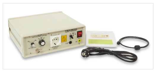
Conducted emissions testing for commercial or consumer products is performed according to the international standards CISPR 11 or 32 and requires a line impedance stabilization network (LISN) between the source of AC line (or DC) voltage and the product under test (Figure 5). The 4/5/6 Series Mixed Signal Oscilloscope is connected to the 50-Ohm port and the conducted RF noise voltage will be displayed. Different model LISNs are made for either AC or DC supply voltage.
Ideally, you’ll set up the test according to the CISPR 11 or 32 standard as illustrated in Figure 7. The equipment under test (EUT) is placed on a wooden table 80 cm high with a ground plane at floor level. The LISN is bonded to the ground plane and connected to the EUT and 4/5/6 Series MSO with Spectrum View.
Troubleshooting conducted emissions will be described in this application note with less detail, because the process is essentially the same as for the radiated emissions test.
Connect a Line Impedance Stabilization Network (LISN), such as the Tekbox TBLC08, and position it between the product or system under test and the 4/5/6 Series MSO with Spectrum View. When troubleshooting on a table top, it’s best to lay down a layer of aluminum foil as a ground plane. Use copper tape to bond the LISN to the foil. Isolate the EUT from the ground plane. Note the sequence of connections in the sidebar!
CAUTION: It’s often important to power up the EUT prior to connecting the LISN to the oscilloscope. This is because large transients can occur at power-up and may potentially destroy the sensitive input preamplifier stage of the oscilloscope. Note that the TekBox TBLC08 LISN has builtin transient protection. Not all do…you’ve been warned!
SETTING UP SPECTRUM VIEW FOR GENERAL CONDUCTED EMISSIONS TROUBLESHOOTING
Using a similar procedure as for radiated emissions, set Spectrum View to display frequencies from zero to 30 MHz. Use a Center Frequency of 15 MHz, Span of 30 MHz and resolution bandwidth of 9 or 10 kHz. Power up the EUT and then connect the 50-Ohm output port of the LISN to the oscilloscope. Note the harmonic frequencies are usually very high at the lower (kHz) frequencies and taper off towards 30 MHz. Be sure these higher harmonic frequencies don’t overdrive the oscilloscope. Adjust the Vertical Scale as needed or on the Tekbox TBCL08 LISN (as shown in lower left of Figure 6), select the transient protector, which includes a 10 dB attenuator.
Spectrum View will capture peak-detected harmonics and the required test limits will be in terms of average or quasi-peak, so you won’t be able to directly compare the measured data to actual test limits. However, you’ll at least be able to determine potential problem areas. The process for troubleshooting harmonic frequencies is similar to the radiated emissions testing described previously.
Analyzing the Collected Data
Remember that not all near field signals will couple to “antenna-like” structures and radiate. Note that in many cases, two, or more, sources will generate some (or all) of the same harmonics. For example, a 25 MHz clock and 100 MHz clock can both produce harmonics of 100, 200, 300 MHz, etc. Oftentimes, you’ll need to fix more than one source to eliminate a single harmonic. Spectrum View includes some powerful data capture and documentation features that will help speed up the data collection process from steps 1 through 3.
After the harmonics are analyzed and you have identified the most likely sources, the next step is to determine the coupling path from source and out of the product. Usually, it’s the I/O or power cables that are the actual radiating structure. Sometimes, it’s leaky seams or apertures (display or keyboard, for example).
There are four possible coupling paths; conducted, radiated, capacitive, and inductive. The latter two (capacitive and inductive) are so-called “near field” coupling, and small changes in distance between source and victim should create large effects in radiated energy. For example, a ribbon cable routed too close to a power supply heat sink (capacitive coupling, or dV/dt) and causing radiated emissions can be resolved merely by moving a ribbon cable further away from a nearby heat sink. The inductive coupling (di/dt) between a source and victim cable can also be reduced by rerouting. Both these internal coupling mechanisms (or similar PC board design issues) can lead to conducted emissions (via power cables) or radiated emissions (I/O or power cables acting as antennas or enclosure seams/apertures). In many cases, it’s simply poor cable shield bonding to shielded enclosures or lack of common-mode filtering at I/O or power ports that lead to radiated emissions.
Often, when troubleshooting emissions, you may have already run a formal compliance test and know how far over limit the harmonics are. So, when troubleshooting, the important point is that relative measurements are generally important, rather than absolute. That is, if we know certain harmonics are 5 to 10 dB over the limit, the goal would be to reduce these by at least that, or more, for a safe margin. Therefore, a calibrated antenna is not required, as only relative changes are important. The antenna also does not necessarily need to be tuned to the frequency of the harmonics. The important thing is that harmonic content from the EUT should be easily visible.
Accounting for Ambient Signals
One problem you’ll run into immediately when testing outside of a shielded room or semi-anechoic chamber is the number of ambient signals from sources like FM and TV broadcast transmitters, cellular telephone, and two-way radio. This is especially an issue when using current probes or external antennas.
If there are just a few harmonics of concern, often, it’s easier to narrow the frequency span on the spectrum analyzer down to “zoom in” on a particular harmonic frequency, thus eliminating most of the ambient signals. A common example is differentiating a 100 MHz clock harmonic from the 99.9 MHz FM broadcast band channel. If the harmonic is narrow band continuous wave (CW) partially hidden among the modulation frequencies, then reducing the resolution bandwidth (RBW) can also help separate the harmonic. Just be sure reducing the RBW doesn’t also reduce the harmonic amplitude as well.
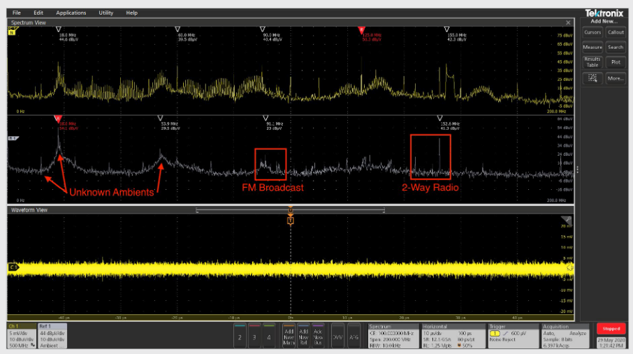
Often, it’s good to see the “big picture” of ambient signals within the entire band of interest. To account for ambient signals using Spectrum View, first turn off the device under test and set up the spectrum limits and Span as desired. For this example, we’ll use a Center Frequency of 100 MHz and a Span of 200 MHz. A resolution bandwidth (RBW) of 10 kHz for general purpose troubleshooting can be a good place to start in order to clearly resolve the harmonics. Then, save the spectrum plot as an ambient baseline by using File > Save As > Ch1 > SV_Normal > then enter a filename > Save (Figure A).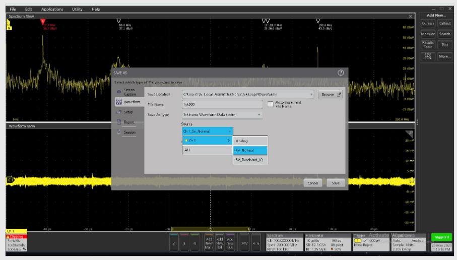
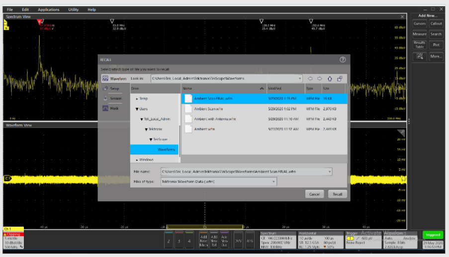
This will record the various broadcast stations, two-way radios, digital TV, and cellular phone signals. Recall the saved waveform using Recall > Waveform > select the Filename > Recall (Figure B). Then, turn on the EUT and save a sweep to record both the ambient and EUT signals. You’ll end up with a screen similar to Figure C.
You’ll notice a lot of activity around the FM broadcast band (88–108 MHz), the digital TV band (470 to 608 MHz), and cellular phone (generally 600 to 850 MHz for bands below 1000 MHz). Refer to Reference 6 for more details on cellular frequency bands within the U.S.
The technique is not foolproof, as there may be additional two-way radio transmissions that are not caught in the ambient capture, but it will still give you a good idea as to what signals are coming from the device under test. To confirm whether a harmonic frequency is from the device being measured, you may need to power it off occasionally.
Time-Correlated Troubleshooting
If you’re unable to stabilize the time domain waveform, and the signal is “messy”, but arrives in fixed bursts (very common for digital bus or IoT/wireless circuits), try measuring the period between bursts and setting the Holdoff time to stabilize the trigger. If this doesn’t work, you can also Stop the acquisition to analyze the stored waveform data.
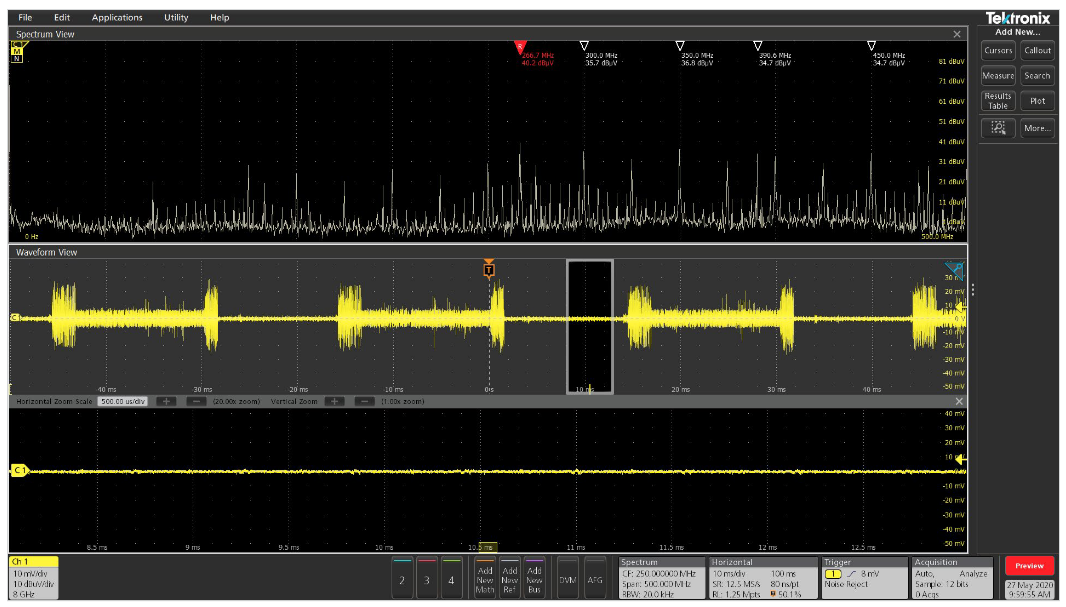
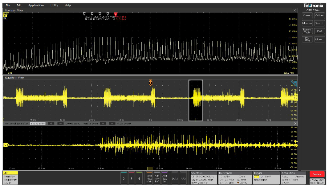
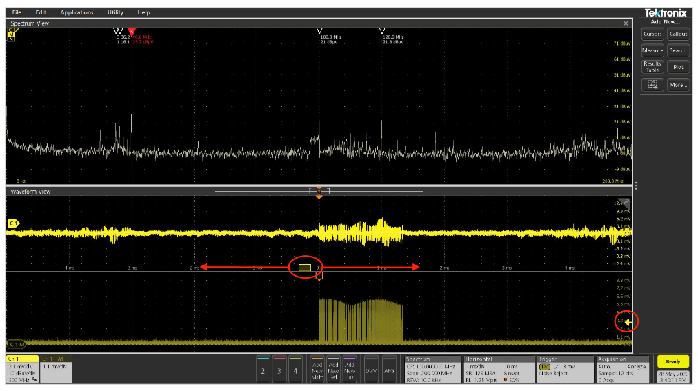
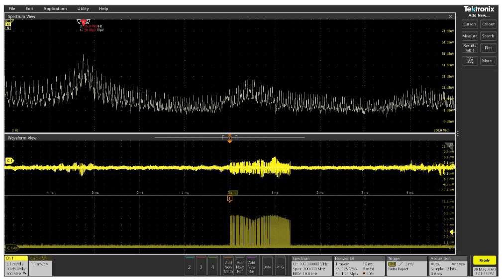
Once you achieve a stable waveform (or have the acquisition stopped) then you can use the Zoom knob (lower-right) turned clockwise to magnify the time domain waveform. This will automatically display the zoomed waveform at the bottom. Notice that Spectrum Time (a colored box of varying size depending on the zoom ratio and RBW) appears on the time domain waveform. By narrowing this down and grabbing it with your finger or mouse, you’ll see the effect on the frequency domain, depending on the box position in the time domain acquisition. By placing it over certain portions of the time domain waveform, you may be able to observe time dependencies on the spectrum plot. See Figures 8 and 9 for examples of Spectrum Time on the oscilloscope’s display.
As an example, we’ll measure the DDR RAM bus noise from a fingerprint scanner used as a secure entry access (Figure 7). There is a flex cable directly adjacent to this memory IC, which is coupling to the data bus and radiating a regular pulse of EMI. Very often a pulse of digital activity can produce strong harmonic content.
Adjust the Horizontal time base such that multiple noise bursts are shown in the time domain screen. Adjust the Trigger Level for a stable display or simply stop the acquisitions using the Run/Stop front panel button (upperright). Then use the Zoom knob (lower-right) turned clockwise to start magnifying the waveform.
Notice the zoom window as it progressively gets shorter as you zoom in. By grabbing this zoom window with the mouse or your finger and sliding it back and forth along the time domain waveform, you’ll be able to see the effect on the harmonics of various portions of the time domain waveform. From this, you may be able to deduce the origin of these bursts and apply some mitigations. Figures 8 and 9 show how the different portions of the time domain waveform affect the harmonic content and how the Spectrum View window updates to show the spectrum content that correlates to the selected Spectrum Time. At the leading edge of the burst, harmonics increase by 20 dB.
Advanced Triggering Techniques
Hardware Triggered Troubleshooting - The Tektronix 4/5/6 Series MSOs have an RF versus Time hardware trigger option enabled by the RFVT option and found within the Trigger badge (RF vs Time trace must be active for trigger option to be presented).
- Magnitude versus Time - displays the RF Magnitude versus Time in a separate plot.
- Frequency versus Time - displays a RF Frequency Deviation versus Time in a separate plot.
- Phase versus Time - displays the RF Phase versus Time in a separate plot.
All three of these may be displayed simultaneously and hardware triggering can be selected for edge, pulse width and timeout events on RF Magnitude vs Time and RF Frequency vs Time plots.
EXAMPLE: MAGNITUDE TRIGGERING
Magnitude versus Time triggering measures the magnitude of the frequency content and allows triggering on magnitude edges, pulse widths and timeout events. This is helpful when the frequency content may correlate to certain harmonic conditions, such as harmonics which pulse upward intermittently.
For example, a 35 MHz harmonic was observed with a medium-sized (1 cm) H-field probe to pulse upward by 30 dB on occasion. This intermittent harmonic could easily result in compliance failure should it couple out to an I/O cable and radiate.
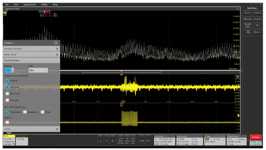
Let’s assume the probe is connected to Channel 1. To set up this special triggering mode, double-click the Channel 1 badge and select Spectrum View. Make sure it is turned ON, and then turn on Normal and Max Hold. Turn on Magnitude in the RF versus Time Waveforms section (Figure 10).
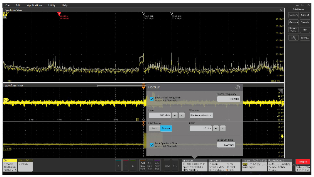
Now double-click the Spectrum controls box towards the lower-right and set a Center Frequency of 100 MHz and Span of 200 MHz. I also prefer the vertical scale to read “dBuV”. This will display a spectrum from zero Hz to 200 MHz. Set the resolution bandwidth (RBW) to 10 kHz, leaving all else to the default settings (Figure 11).
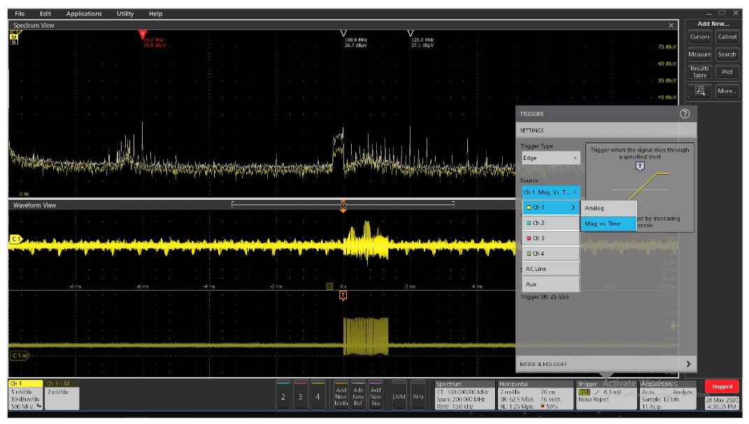
Finally, double-click the Trigger controls (bottom-right) and set the Trigger Type to Edge (default), the Source to Channel 1 and hovering the mouse or a single tap with your finger will show the choice “Mag_vs_Time” and select it (Figure 12). Make sure that “Mag_vs_Time” and Spectrum View are set up, otherwise this option will not be present. Now type in the desired trigger value or position the “Channel1-Mag” plot so its visible and adjust the yellow arrowhead (within the vertical scale) upwards until the trigger reference line is above the noise and somewhere within the magnitude pulse.
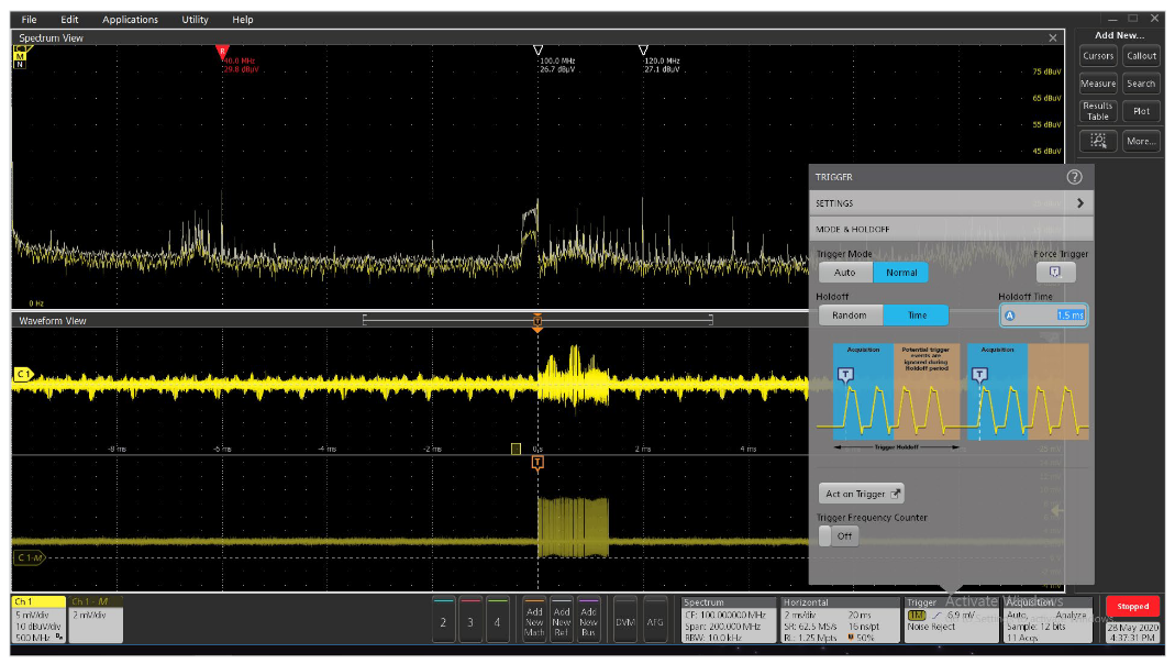
If the digital pulses are spaced widely apart, you may need to adjust the Trigger Holdoff. Within the Trigger panel, select “Mode and Holdoff”, set the Trigger Mode to Normal, the Holdoff to Time, and set the Holdoff Time to something larger than the pulse width you are isolating. In this case, the pulse width was about 1.3 ms, so the holdoff time was set to 1.5 ms to ensure the trigger would reset long after the pulse (Figure 13).
Notice the small yellow box along the horizontal axis of the time domain plot. This is the Spectrum Time selector, and its width is dependent on the RBW. By grabbing the Spectrum Time box and sliding it back and forth along the time domain plot, you will observe the frequency changes at different times in the spectral display
For example, with the box slid outside the pulse, the harmonics are at a minimum (Figure 14) and with the box slid into the start of the pulse, the harmonics reach a maximum (Figure 15). The higher the RBW, the wider the Spectrum Time box, but the less the resolution, so you may need to experiment to optimize the analysis for your system.
By plugging in an oscilloscope probe to Channel 2 and probing around your board, you should find other digital signals that correlate to the pulses on Channel 1 and determine whether coupling to cables or enclosure seams is an issue for this 35 MHz harmonic and what mitigations might be best suited to reduce any couplings.
EXAMPLE: FREQUENCY DEVIATION TRIGGERING
Frequency Deviation versus Time triggering measures the frequency deviation of the time domain plot and allows triggering on the deviation (Hz). This is helpful when the frequency domain may correlate to certain harmonic conditions.
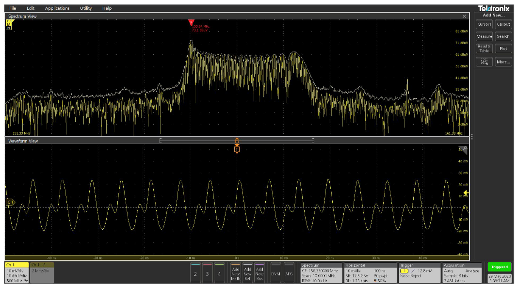
For this example, I discovered a spurious oscillation at about 155 MHz from an op-amp that was terminated poorly and oscillating at its open loop frequency. I could tell it was a classic spurious oscillation, because touching the area caused the frequency to change due to my additional body capacitance.
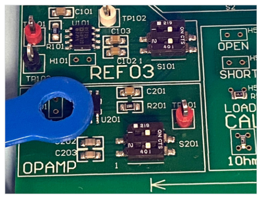
Using the medium-sized H-field probe in Channel 1 and laying it on top of the op-amp, let’s characterize the oscillation (Figure 16). For ease in following the procedure, start by pressing the Default Setup button (lower-right on front panel). Then press Autoset (next to Default Setup) to get a stable time domain waveform without clipping. Double-click the Channel 1 badge to open up Spectrum View panel. Turn the Display ON and turn on the Normal and Max Hold boxes.
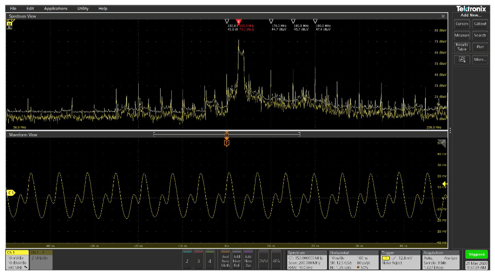
Next, open the Spectrum View settings and set the Center Frequency to 150 MHz and Span to 200 MHz, with RBW set to 10 kHz. We can observe the oscillation clearly at 155 MHz (Figure 17).
Let’s zoom in on the spurious oscillation by opening the Spectrum View settings and selecting a Span of 10 MHz and RBW of 500 Hz, so we can clearly see the frequency response. You may need to move the oscillation back into view by dragging the Spectrum View to center the oscillation in the display (Figure 18).
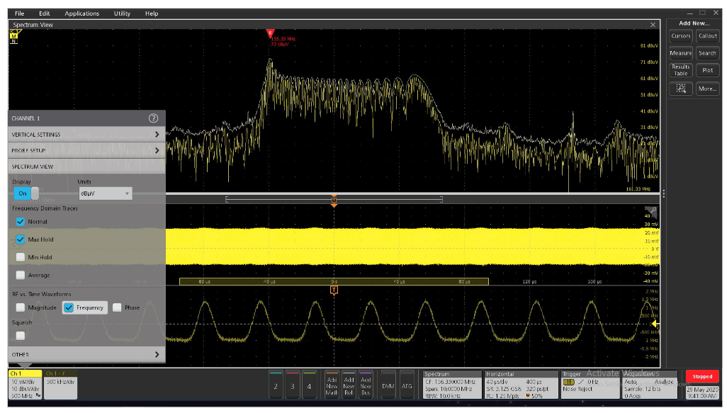
Now go back to the Channel 1 >> Spectrum View panel and select Frequency in the RF versus Time section. You’ll need to adjust the Vertical Scale of the waveform and slow down the Horizontal Scale time base to 40 us/div so its easily viewable. This will display the Frequency Versus Time plot of the oscillation (Figure 19).
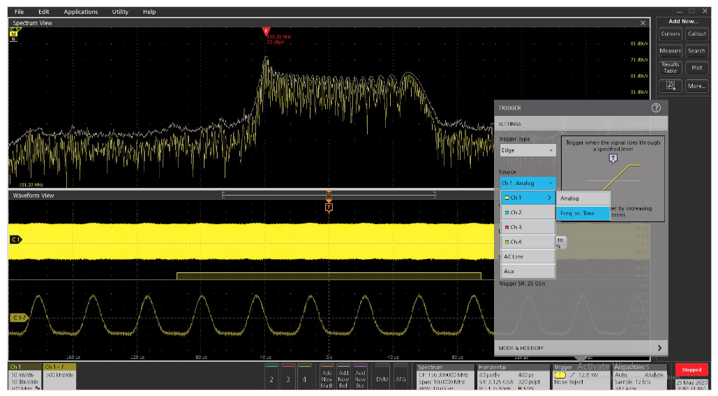
Now, open the Trigger panel and select Channel 1 >> Freq_vs_Time (Figure 20). This will allow triggering on the frequency deviation versus time waveform at the bottom of the display. Adjust the trigger level (yellow arrowhead) to stabilize the RF frequency vs time waveform on your display. You can also optionally stop the acquisitions using the Run/Stop button (upper-right).
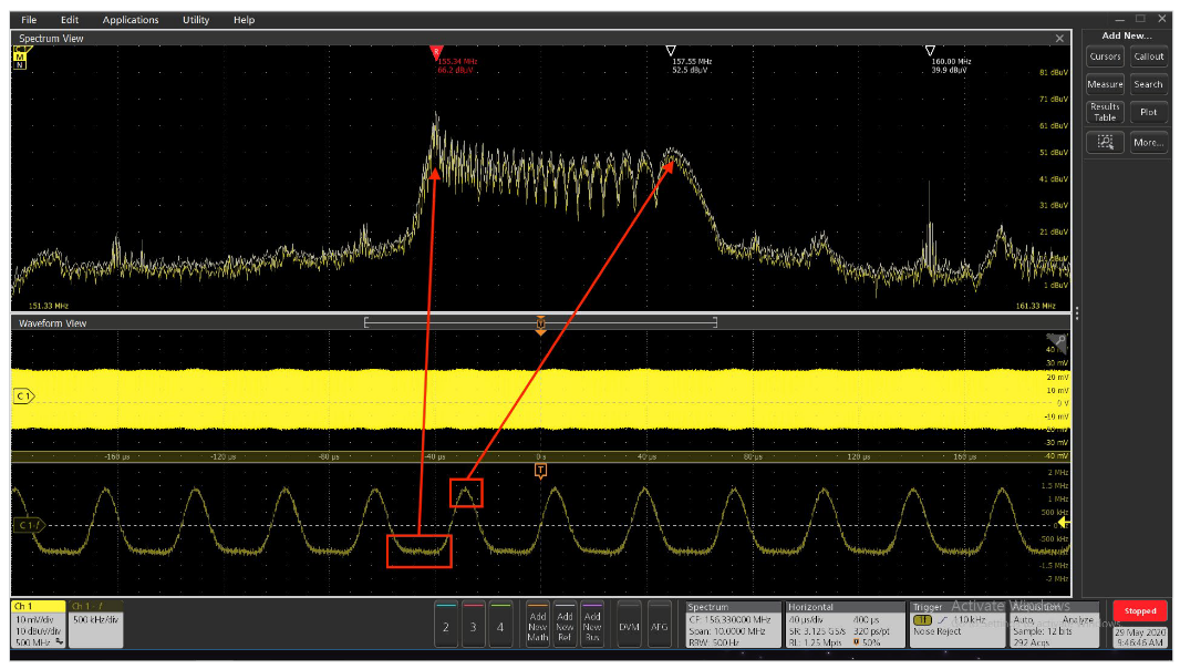
Note that the lower peak at 155.34 MHz is higher than the right-hand peak at 157.55 MHz (Figure 21). Examining the frequency versus time plot at the bottom of the screen shows a peak deviation of about +1.5 MHz and a lower deviation of –1 MHz. This difference approximately corresponds to the difference between the two end peak frequencies as shown by the markers of 157.55 – 155.34 = 2.21 MHz. Observe that the frequency deviation plot (red boxes) lingers at the lower –1 MHz more so than at the +1.5 MHz, which is why the lower frequency peak is higher than the other. All standard time and frequency measurements can be added to the RF vs Time plot and displayed in the measurement results badge on the right of the screen.
In the end, the spurious oscillation was easily controlled by adding output capacitance at the op-amp to control the open-loop gain. This example does show the power of the frequency deviation versus time trigger in helping analyze the characteristics of an unusual harmonic signal that varies in frequency. This would also be a powerful technique for characterizing spread spectrum clock signals.
Summary
By combining the Tektronix 4, 5 and 6 Series MSOs with integrated Spectrum View multi-domain analysis and the time versus frequency triggering, you’ll be able to capture elusive EMC issues faster and easier. By developing your own EMI troubleshooting test lab for radiated and conducted emissions, you’ll save time and money by moving the troubleshooting process in-house. This will save you time and cost when compared to performing troubleshooting at commercial test labs.
As technology continues to advance, we EMC engineers and product designers need to upgrade our usual analysis test tools to stay one step ahead and be able to better capture and display the more unusual emissions expected. Oscilloscopes, such as the 4/5/6 Series MSOs, with time-corelated or hardware (amplitude or frequency) triggering have already proven to be invaluable for EMI debug and troubleshooting. Advanced spectral analysis will be especially important as mobile devices continue to shrink and more products incorporate wireless and other advanced digital modes.