Abstract
Stressed eye testing allows the introduction of different kinds of jitter components. How can the user tell whether the right amount is being introduced? What will different components look like when measured with deep BER-based jitter analysis? This paper examines these questions using the BERTScope S 12500A as the basis.
1. Introduction
Stressed eye receiver testing, or receiver jitter tolerance testing to give it its proper name, is an increasingly common method of evaluating the performance of receivers[i]. The construction of the stressed eye requires a variety of different impairments to be added together, depending upon the standard. A big issue in stressed-eye testing has always been the calibration of the individual stress impairments to ensure that tests comprise enough impairment to ensure compliance is properly being tested, but not so much that good components are failed because the testing was too stringent. Recently introduced stressed-eye test sets eliminate the need for racks of equipment and complex calibration processes. Here, we are going to look at how stress may be evaluated, and how it will appear on the commonly used BER-based Jitter Peak, or BERTScan measurement of jitter[ii]. Measurements used as examples are mainly taken from a BERTScope BSA125C (Figure 1.1).
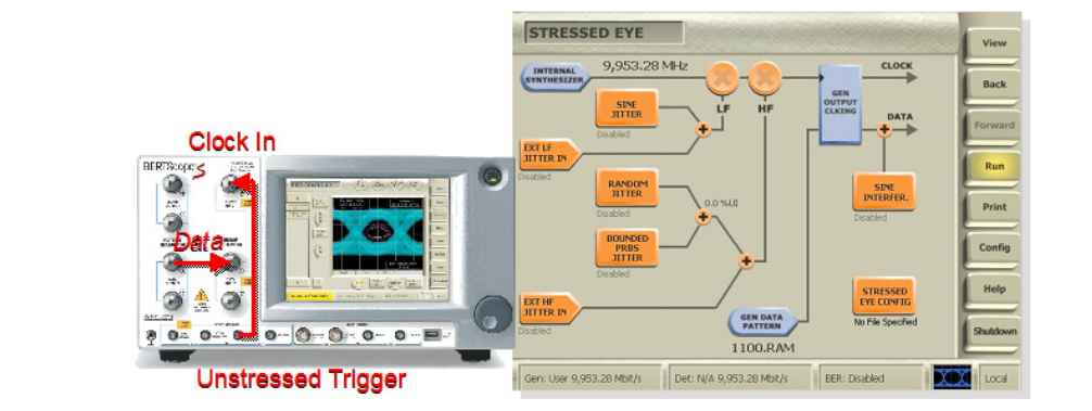
The method we are going to examine in this paper is shown in Figure 1.2. It has the advantage of being simple and requiring no external test equipment. It relies on a BER-based instrument's unique ability to measure total jitter directly and accurately[iii].
2. Simplifying the Problem
The average eye crossing point is complex (Figure 2.1). When measured, it will be composed of the combined effects of random events (noise), inter-symbol interference, crosstalk, and various other effects including random and deterministic effects from the measuring equipment itself.
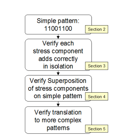
In order to see what is going on, it is common to simplify the problem. To take out deterministic effects of the measurement system, it is useful to go back to basics. Patterns such as 11001100 and 10101010 look like square waves, and are the simplest that data can get (see Figure 2.2). Using such patterns eliminates pattern-related effects. For this paper we will use a 11001100 pattern.
Having removed pattern-related effects, the next step is to examine each impairment individually, without complication except for the intrinsic effects of the test equipment.
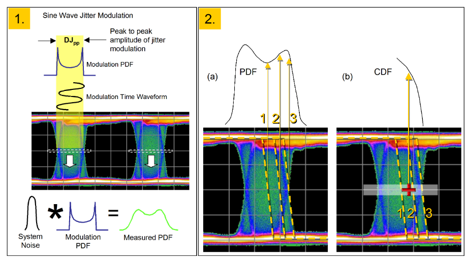
Before looking at how individual jitter types might appear when measured using BER-based jitter measurements, it is worth doing a brief recap of jitter measurements and how they appear on different instrument types. A common method of looking at jitter is by examining an eye diagram and measuring the number of hits that occur around the eye crossing point (white dotted line box in Figure 2.3 (1)). A second method is to use a BER-based instrument and to scan the decision point across the eye at the level of the eye crossing point (Figure 2.3 (2)(b)). The first method yields a histogram of jitter, also called a PDF or probability density function – the probability of an edge being at a particular position. The second method yields a cumulative distribution function, or CDF. This is different than a PDF, as illustrated in Figure 2.3 (2). With a PDF, edges 1, 2 and 3 contribute to different parts of the histogram. With a CDF, it is the distribution of BER across the eye – a decision point placed at the position of the red cross will record errors because of edges occurring at that point, and all edges occurring to the right of that point also - in other words, edges 2 and 3 both contribute to the BER at that point. This is why it is termed cumulative. The CDF is the result of measurements known as BERT Scan1 , Bathtub jitter and Jitter Peak. A more detailed explanation of these concepts is given in reference [ii].
Referring to Figure 2.3(1), this illustrates the way different PDFs contribute to a measured eye histogram PDF. The diagram shows a sine wave modulation in the time domain, with its PDF. This is transferred onto the edges of the data signal. This idealized modulation PDF then becomes combined with the real noise in the system to produce the convolved PDF that would actually be measured.
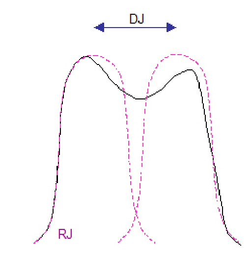
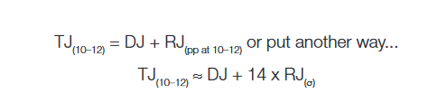
The dual-Dirac model of jitter sub-component separation takes a measured PDF and assumes a random jitter portion that follows a Gaussian distribution has been convolved with a simple theoretical model of 2 Dirac functions representing the deterministic portion. It fits a Gaussian profile to the leading and trailing edge of the PDF, and takes the separation of the means of each of the two Gaussian profiles resulting from the convolution of the random jitter portion with the simple deterministic portion to represent the deterministic effects. This is shown in simplified form in Figure 2.4. The main aim of the dual-Dirac model is to be able to separate simple deterministic and random effects and to extrapolate total jitter measurements, TJ(BER), down to required BER level, usually 1x10–12, TJ(10–12)
where RJ(σ) is the standard deviation of the Gaussian (or RMS value), and 14 is the frequently used approximation of 14.069 which is a standard relationship of Gaussians between standard deviation and peak-to-peak at probability level of 1x10–12[vi].
While the model is good for TJ, it is strongest at RJ/DJ separation when there is either RJ alone, or mainly DJ and small amounts of RJ. More detail on why this is the case is given in reference [ii].
The math is a little different when applied to a CDF, but the concepts are the same. A CDF is usually plotted on a log scale. We will use these ideas to further explore how different types of stress modulation might appear when measured using a BER-based measurement such as Jitter Peak. Using the ideas of PDFs and CDFs leads to Figure 2.5, where we are going to look at how some stress types might appear as PDFs and then how they might be measured on a BER-based jitter measurement such as Jitter Peak.
The easiest to understand is modulating data edges with a square wave, as shown in Figure 2.5 (1). While this isn't a common form of stress modulation, it is useful as a starting point. A square wave theoretically spends all of its time either at the ‘one' level, or the ‘zero' level, with almost no time transitioning between. This means that plotting a probability density function (PDF) of the position of the edges should be almost a pair of delta or Dirac functions, as shown in the diagram.
Sine wave jitter is similarly easy to understand. A sine wave spends more time in between extremes than a square wave, but still spends more time at extremes than in the mid-portion as the modulation dwells as it changes direction, and is at its fastest through crossing the center. Figure 2.5 (2) shows this. Again, the net result is that the Jitter Peak measurement is dominated by DJ, with the main RJ contribution being mainly the instrument intrinsics.
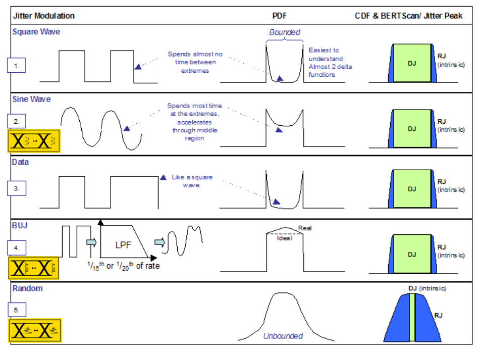
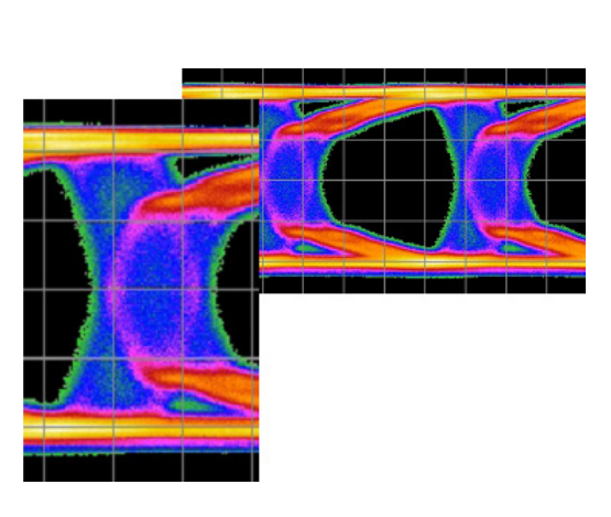
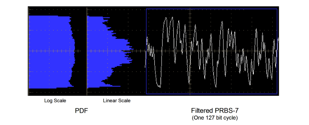
Using the logic of the square wave case, data would have a similar PDF and Jitter Peak (Figure 2.5 (3)). Bounded Uncorrelated Jitter (BUJ) is designed to emulate crosstalk and other interference, which is data that is uncorrelated to the signal under test but that has a similar spectrum. Ideally, it is supposed to have a PDF that is rectangular, with any edge position being equally likely. In practical terms this is not achievable, but taking a PRBS signal (typically PRBS7) at a data rate unrelated to the signal under test to avoid beating effects (for example 2 GHz for a 9.953 Gb/s test) and then passing the modulation signal through a low pass filter (LPF) at 1/15th or 1/20th of the modulation rate does get near to the desired PDF (Figure 2.5 (4) and a real measured example in Figure 2.6). Again, the result in dual-Dirac terms is a Jitter Peak dominated by DJ with only the intrinsic RJ of the measuring instrument present in addition.
Note that all of the modulations discussed so far have bounded PDFs — edges have a particular probability of occurring at any position within finite limits, and zero probability of appearing outside of these limits. This is not the case for truly random modulation of edges (Figure 2.5 (5)). In this case the Jitter Peak is almost entirely composed of random jitter, with just a small contribution from any inherent DJ of the measuring equipment.
3. How is the BERTScope Stress Calibrated?
A BERTScope is able to generate stress and measure itself with a Jitter Peak analysis. We are going to continue with the conditions we've just been discussing — a 11001100 data pattern and a single source of jitter modulation at a time — and look at each modulation type.
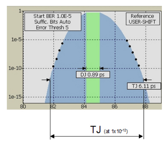
The overall strategy of calibration is to make the jitter component make sense down at 1x10–12 BER, which is where almost all jitter standards require measurements to be made (Figure 3.1). Dual-Dirac measurements such as Jitter Peak give the total jitter (TJ) width at this level, and also an estimate of random (RJ) and deterministic (DJ) sub-components. As stated earlier, TJ is the most trustworthy and accurate measure, and is not impacted by limitations of RJ and DJ separation that can become evident under certain conditions with the dual-Dirac model.
For DJ-related modulation components, the BERTScope is calibrated to take account of the intrinsic jitter of the instrument at each data rate, and to add the required amount of jitter to increase the total jitter by the correct amount. For example, if the TJ of the instrument measured back-to-back is 6% UI, and 10% SJ modulation is applied, the TJ should increase to 16%.
This method of providing calibrated results is true for all of the DJ-related modulation components. RJ addition is slightly different. It is assumed that the intrinsic jitter of the instrument is dominated by RJ rather than DJ. If the user requests 10% RJ to be provided, the instrument will add the required amount of RJ to end up with the right TJ value. Using our example above, more RJ will be added to end up with the requested 10% RJ2 . The intrinsic levels vary with operating frequency, and the factory measured levels are held in a calibration table.
Let's look at some examples. In each case, graphs are shown for 11001100. In some cases, graphs are used that were taken from an instrument with unspecified calibration. They are provided because they are useful for examining the RJ/ DJ component behavior of TJ. Note that these graphs have a jitter axis displayed in ps — as the measurements were carried out at 9.95 Gb/s (to within 0.5%), these figures also equate to %UI. Note also that the measured values of RJ were displayed as RMS values, they have been multiplied by 14 on the graphs to translate them to peak-to-peak values at 1 x 10–12 to aid comparison and place them on a par with the DJ values.
Measured Sinusoidal Jitter (SJ) Example
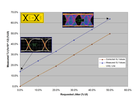
To illustrate the concepts described above, we measured a BERTScope with different applied SJ levels. The intrinsic TJ was about 13.9% UI at this bit rate on this instrument. SJ is applied as shown in Figure 3.2, in 10% increments. The Jitter Peak measurement has been used to measure the total jitter, TJ (upper, blue line). For illustration purposes, the intrinsic jitter offset has been subtracted (lower, brown line). A unity line has also been inserted (yellow line) to enable deviation from ideal to be observed.
Note that the eye diagrams shown for illustrative purposes also have jitter measurements displayed. These are inadequate for jitter calibration because scope eye diagrams are inherently based on much shallower data, and so do not give the correct TJ. For DJ-related stress modulations, they should approximately track the correct values. SJ jitter is the component that most requires high accuracy, as it must follow precise jitter templates in stress testing.
Measured Bounded Uncorrelated Jitter (BUJ) Example
A BUJ example is shown in Figure 3.3. BUJ is produced by modulating the normal clock transitions with a pseudo-random sequence meant to mimic cross-talk in a real-world situation. For this example, the BUJ modulation is based around a PRBS-7 modulation. Once again, the intrinsic jitter of the instrument is added to in steps (of 10% for this example).
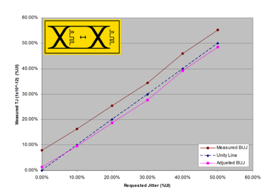
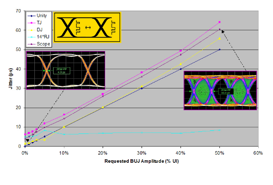
Figure 3.4 shows the RJ and DJ subcomponents separated using Jitter Peak. Note that the eye diagram-based jitter measurements (labeled ‘scope') are lower than the TJ values. Again, since eye diagram measurements are based on shallower data, the full effects of low probability events (in this case intrinsic RJ) are missed. However, as the added jitter is high-probability deterministic jitter, the eye diagram captures it fairly well and the results track TJ fairly well. In the graph, RJ remains at approximately its intrinsic level, and almost all of the added jitter shows as DJ. Note that the convolution of noise (RJ) with BUJ (DJ) causes the means of the Gaussians of the model to move towards each other, as discussed earlier. Since real modulation DJ does not equate to a pair of Dirac delta functions, the model will deviate from expected levels of DJ. This is why texts refer to two different DJs — DJ(pp), which is the peak-to-peak amplitude of the applied modulation, and DJ(δδ) , which is the measured DJ, the distance between the two Dirac delta functions of the dual Dirac jitter model.
For square wave modulation that approximates a PDF of two delta functions, the values will be the closest. For modulation such as BUJ the PDF is a long way from being a pair of Dirac delta functions, and DJ(δδ) will be significantly less than DJ(pp). Because of these issues, the BERTScope is always calibrated using TJ measurements so that the correct amount of DJ is applied to the internal modulators (whatever value it needs to be) in order to get the correct TJ(10–12)
Measured Random Jitter (RJ) Example
As already stated, RJ is different to other impairments for a number of reasons. As shown in Figure 3.5, at low levels of RJ, the instrument's own intrinsic RJ dominates and already exceeds the requested value. Under these conditions the instrument warns the user as such, and adds no extra RJ.Once the requested RJ exceeds the intrinsic level, RJ is added to end up with the correct amount of TJ.
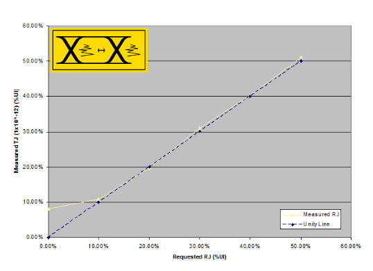
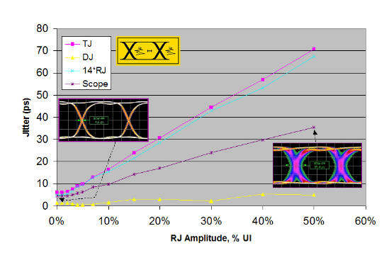
Figure 3.6 shows a set of results taken with the uncalibrated instrument, useful for illustration purposes. Here the jitter subcomponents taken as part of the TJ measurement are plotted, as is the eye diagram jitter measurement. As predicted from Figure 2.3, it can be seen that most of the added jitter comes from RJ, with only a small amount of intrinsic DJ present. Note that the eye diagram based jitter measurement misses a large proportion of the total jitter, as it is based on a shallow sample depth measurement. Here the eye-based measurement does not track TJ in the same way as in the DJ cases, and this demonstrates the inherent advantage of a BER-based measurement over an eye-based measurement.
Measured Sinusoidal Interference (SI) Example
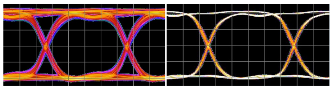
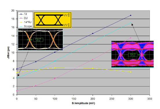
A common impairment not yet mentioned is Sinusoidal Interference (SI). SI is an impairment intended to close the eye down in the vertical, amplitude dimension. However, as can be seen from the right-hand screenshot of Figure 3.7, amplitude closure on signals with finite rise times also translates into increased jitter. Figure 3.7 shows the effect on measured jitter of increasing amounts of SI. SI is bounded in nature, and in the jitter domain behaves approximately like SJ. Hence the eye diagram based jitter measurements track the TJ, as seen before for other deterministic-dominated stress components.
4. Adding Two Impairments at the Same Time
The situation gets more complicated when more than one stress impairment is involved at a time. Keeping with the 11001100 pattern for simplicity, we are going to examine the effect of having one fixed level impairment, and introducing a second one at differing levels to show superposition.
First of all, it is worth having a quick reminder of how PDFs combine. For simplicity, we're going to assume that we are going to be combining two stress components with the same ‘rectangular' PDFs (Figure 4.1). As the two convolve together, the resulting distribution has the same area as either one (the probability of the edge falling somewhere in time is still 1), but a very different distribution. The combined distribution is still bounded but has tails that are at lower probability of occurrence. As may be remembered, as more distributions of similar significance are added together, the more the resulting distribution approaches a Gaussian (the Central Limit Theorem). In reality, if we were to do the experiment of Figure 4.1 with very simple distributions as shown, we would already also be convolving the intrinsic DJ and intrinsic RJ of the measuring system as well, so it becomes obvious that the resulting distribution will be more and more Gaussian-like.
Real stress components do not have the simple rectangular distribution PDFs shown in Figure 4.1. It therefore makes predicting exactly what the resulting distribution will be when two components are added together difficult in practical terms. It is easier to verify with measurement, as we are about to see.
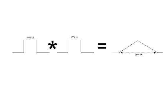
Figure 4.2 shows what happens when a single BUJ stress component, set to 20% UI, has a second component added. In this example it is an SJ signal that is varied from 0 to 55%. Both contributions are also classed as PJ, or periodic jitter. We are combining two contributions that affect DJ almost entirely. As might be expected, the BUJ behaves as an offset, and the SJ builds on top of that. The RJ contribution is roughly flat. Note that the graph shown starts at 5% added SJ. It is useful to look at the missing part of the graph in more detail.
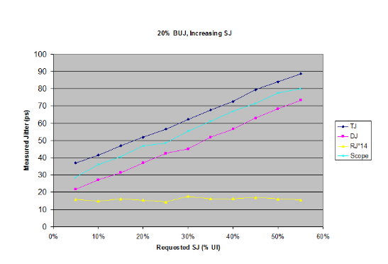
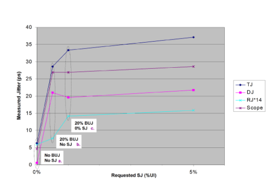
Figure 4.3 shows the left hand end of the graph of Figure 4.2, the part that is missing. For illustration purposes the SJ values have been altered — in reality, the left three sets of data points should all be at 0% SJ, but this makes viewing difficult.
Figure 4.3 (a)
The left-most set of data points ("a") are for the case where no stress is switched in. The jitter present is the intrinsic jitter of the instrument, which is mostly RJ with a small amount of DJ. Stress is added using two separate modulators — one able to provide many UI of jitter that is used for SJ insertion ("LF Modulator"); the second is used for RJ and BUJ ("HF modulator" — see Figure 4.4).
Figure 4.3 (b)
The next set of data points, "b" in Figure 4.3, are for the 20% BUJ being switched in. This has activated one of the two modulators in the instrument, and the TJ has increased significantly as expected. Note that the DJ has increased, which is logical for a deterministic stress component. However, the RJ has also increased because of the addition of more active circuitry into the data path.
Figure 4.3 (c)
This is even more apparent when the second modulator is switched on, even though it is not being used for the addition of SJ yet ("c"). Here the TJ has increased along with the measured RJ, even though no more deliberately introduced jitter is being added. The modulator used for SJ is expected to be able to operate over many UI of jitter, unlike the first one. It is composed of multiple stages of active components, and considerable care has been taken with the BERTScope design to ensure that the inherent RJ is low.
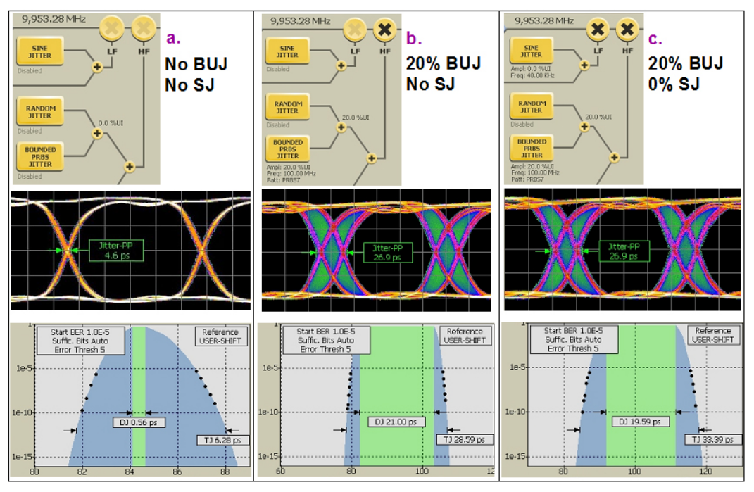
The results of Figure 4.3 are shown from different perspectives in Figure 4.4. The top-most part of the figure shows the status of the modulators for each measurement. The bottom part shows the Jitter Peaks for each. Jitter Peak "a" shows the intrinsic jitter of the particular machine used, with no modulators switched on. "b" (rescaled) shows the added 20% BUJ as DJ (green region). "c" is the same as "b" except that the second modulator is active but not being used. More RJ is now present, as seen in the increased width of the blue regions. The middle set of screenshots is the associated eye diagrams that go along with these measurements. Note that the shallow eye-based jitter measurement doesn't see the increased RJ between "b" and "c".
5. Translating to Real World Test Signals
Testing individual stress components on simple patterns such as 11001100 is a great way of seeing what effect you are having; it minimizes the effect of other non-ideal responses in the overall system, and is the most accurate way to verify that each impairment is sufficiently well-calibrated.
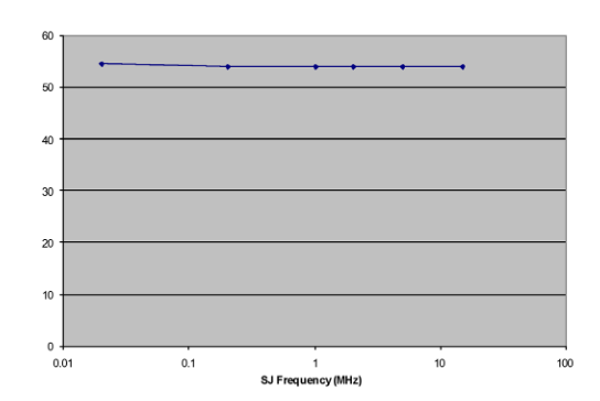
The first pragmatic point to make is that amplitudes, once set, should remain constant when other parameters such as modulation frequency are changed. Figure 5.1 shows amplitude stability of a particular measurement setup. SJ was set to a nominal value of 10% UI, and the TJ measured with Jitter Peak. The modulation frequency was then changed, and TJ re-measured. The pattern was a PRBS-7, and in this example the level stays constant to better than 0.1 dB.
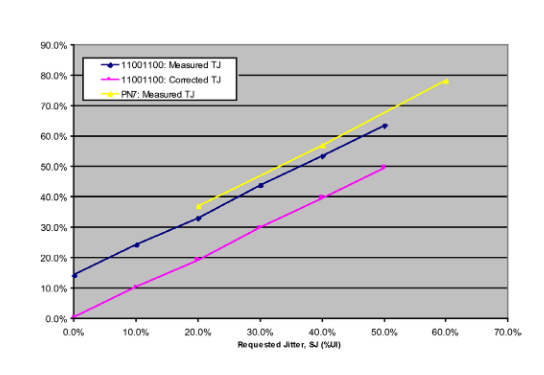
A second necessary step is to verify that if jitter behaves as expected with a 11001100 pattern, the same applies for more real-world patterns. This is shown in Figure 5.2. Here, the data of Figure 3.2 showing TJ measurements with applied SJ for a 11001100 pattern is re-plotted alongside equivalent measurements for a PRBS-7. As can be seen, the measurements track. As the PRBS-7 pattern excites other jitter mechanisms, the overall TJ values are higher, as expected. Similar results for a different measurement set are shown in Figure 5.3. Here, the test signal was at a data rate of 4.25 Gb/s, and the measured values are in ps rather than %UI.
6. Summary
We've looked at how jitter measurements may be self-verified using a BER-based Jitter Peak measurement. We've simplified the measurement challenge by using a pattern that does not contribute pattern-dependent effects, and shown how different stress impairments contribute to the total jitter (TJ). We have explained some of the limitations of the dual-Dirac jitter model. We have also seen how each impairment is calibrated, as well as how each contributes RJ and DJ components. Lastly, we have translated these results over to more real-world signals.