XYZ's of Oscilloscopes

Evaluating Oscilloscopes
Once you understand what an oscilloscope is and have determined the type of oscilloscope you need, there are still many models to choose from, including portable and hand-held. And when choosing an oscilloscope, there are a number of things to consider, such as the ease-of use, sample rate the probes used to bring data into it, and all the elements of an oscilloscope that affect its ability to achieve the required signal integrity.
To understand these considerations, we'll look briefly at ease-of-use and oscilloscope probes, and then describe some useful measurement and oscilloscope performance terms. These terms cover the criteria essential to choosing the right oscilloscope for your application.
Ease-of-Use
Oscilloscopes should be easy to learn and easy to use, helping you work at peak efficiency and productivity. This means you can focus on your design, rather than the measurement tools. Just as there is no one typical car driver, there is no one typical oscilloscope user. Regardless of whether you prefer a traditional instrument interface or a Windows® software interface, it is important to have flexibility in your oscilloscope's operation. Many oscilloscopes offer a balance between performance and simplicity by providing many ways to operate the instrument. A typical oscilloscope's front-panel layout (Figure 60) provides dedicated vertical, horizontal and trigger controls.
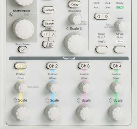
Figure 60: Traditional, analog-style knobs control position, scale, intensity, etc. – precisely as you would expect.
The Complete Measurement System Probes
Even the most advanced instrument can only be as precise as the data that goes into it. A probe works in conjunction with an oscope as part of the measurement system. Precision measurements start at the probe tip. The right probes matched to the oscilloscope and the device under test (DUT) not only allow the signal to be brought to the oscilloscope cleanly, they also amplify and preserve the signal for the greatest signal integrity and measurement accuracy. Please refer to the Tektronix ABCs of Probes Primer for more information about probes and probe accessories.
Bandwidth
Bandwidth determines an oscilloscope's fundamental ability to measure a signal. As signal frequency increases, the capability of an oscope to accurately display the signal decreases. The bandwidth specification indicates the frequency range that the oscilloscope can accurately measure.
Oscilloscope bandwidth is specified as the frequency at which a sinusoidal input signal is attenuated to 70.7% of the signal's true amplitude, known as the –3 dB point, a term based on a logarithmic scale, as shown in Figure 44.
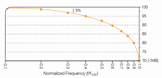
Figure 44: Oscilloscope bandwidth is the frequency at which a sinusoidal input signal is attenuated to 70.7% of the signal's true amplitude, known as the -3 dB point.
Without adequate bandwidth, an oscilloscope cannot resolve high-frequency changes. Amplitude is distorted. Edges vanish. Details are lost. All the features, bells and whistles in your oscilloscope will mean nothing.
To determine the oscilloscope bandwidth needed to accurately characterize signal amplitude in your specific application, apply the “5 Times Rule”:
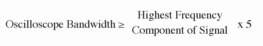
5 Times Rule
An oscilloscope selected using the “5 Times Rule” provides less than ±2% error in your measurements. This is typically sufficient for today's applications. However, as signal speeds increase, it may not be possible to achieve this rule of thumb. Keep in mind that higher bandwidth will likely provide more accurate reproduction of a signal, as shown in Figure 45.
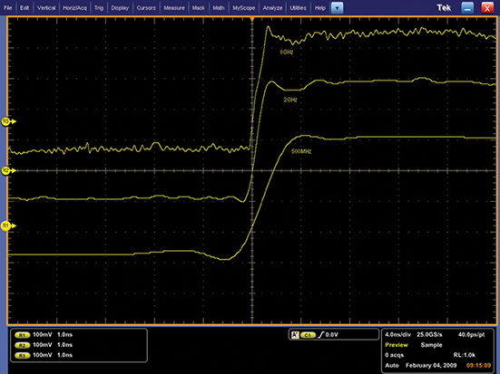
Figure 45: The higher the bandwidth, the more accurate the reproduction of your signal, as illustrated with a signal captured at 250 MHz, 1 GHz and 4 GHz bandwidth levels.
Some oscilloscopes provide a method of enhancing the bandwidth through digital signal processing (DSP). A DSP arbitrary equalization filter can be used to improve the oscilloscope channel response. This filter extends the bandwidth, flattens the oscilloscope's channel frequency response, improves phase linearity, and provides a better match between channels. It also decreases rise time and improves the time domain step response.
Rise Time
Rise time describes the useful frequency range of an oscilloscope. Rise time measurements are critical in the digital world. Rise time may be a more appropriate performance consideration when you expect to measure digital signals, such as pulses and steps. An oscilloscope must have sufficient rise time to accurately capture the details of rapid transitions (Figure 46).

Figure 46: Rise time characterization of a high-speed digital signal.
To calculate the oscilloscope rise time required for your signal type, use this equation:

Oscilloscope Rise Time
Using this equation is similar to using the equation for bandwidth. As in the case of bandwidth, achieving this rule of thumb may not always be possible given the extreme speeds of today's signals. Always remember that an oscilloscope with faster rise time will more accurately capture the critical details of fast transitions.
In some applications, you may know only the rise time of a signal. A constant allows you to relate the bandwidth and rise time of the oscilloscope using this equation:

Bandwidth and Rise Time
Where K is a value between 0.35 and 0.45, depending on the shape of the oscilloscope's frequency response curve and pulse rise time response. Oscilloscopes with a bandwidth of <1 GHz typically have a 0.35 value, while oscilloscopes with a bandwidth of> 1 GHz usually have a value between 0.40 and 0.45.
Some logic families produce inherently faster rise times than others (Figure 47).

Figure 47: Some logic families produce inherently faster rise times than others.
Sample Rate
Sample rate is specified in samples per second (S/s). It defines how frequently a digital oscilloscope takes a snapshot or sample of the signal, analogous to the frames in a movie. The faster an oscilloscope samples (i.e., the higher the sample rate), the greater the resolution and detail of the displayed waveform and the less likely that critical information or events is lost (Figure 48).

Figure 48: A higher sample rate provides greater signal resolution, ensuring that you'll see intermittent events.
The minimum sample rate may also be important if you need to look at slowly changing signals over longer periods of time. Typically, the displayed sample rate changes with changes made to the horizontal scale control to maintain a constant number of waveform points in the displayed waveform record.
How do you calculate your sample rate requirements? The method differs based on the type of waveform you are measuring, and the method of signal reconstruction used by the oscilloscope.
In order to accurately reconstruct a signal and avoid aliasing, the Nyquist theorem states that the signal must be sampled at least twice as fast as its highest frequency component. This theorem, however, assumes an infinite record length and a continuous signal. Since no oscilloscope offers infinite record length and, by definition, glitches are not continuous, sampling at only twice the rate of highest frequency component is usually insufficient.
In reality, accurate reconstruction of a signal depends on both the sample rate and the interpolation method used to fill in the spaces between the samples. Some oscilloscopes let you select either sin (x)/x interpolation for measuring sinusoidal signals, or linear interpolation for square waves, pulses and other signal types.
For accurate reconstruction using sin (x)/x interpolation, your oscilloscope should have a sample rate at least 2.5 times the highest frequency component of your signal. Using linear interpolation, the sample rate should be at least 10 times the highest frequency signal component.
Some measurement systems with sample rates to 10 GS/s and bandwidths to 3+ GHz are optimized for capturing very fast, single-shot and transient events by oversampling up to 5 times the bandwidth.
A Note About Bandwidth and Sample Rate
The digital approach means that the oscilloscope can display any frequency within its range with stability, brightness, and clarity. For repetitive signals, the bandwidth of the digital oscilloscope is a function of the analog bandwidth of the front-end components of the oscilloscope, commonly referred to as the –3 dB point. For single-shot and transient events, such as pulses and steps, the bandwidth can be limited by the oscilloscope's sample rate.
Waveform Capture Rate
All oscilloscopes blink. That is, they open their eyes a given number of times per second to capture the signal, and close their eyes in between. This is the waveform capture rate, expressed as waveforms per second (wfms/s). While the sample rate indicates how frequently the oscilloscope samples the input signal within one waveform, or cycle, the waveform capture rate refers to how quickly an oscilloscope acquires waveforms.
Waveform capture rates vary greatly, depending on the type and performance level of the oscilloscope. Oscilloscopes with high waveform capture rates provide significantly more visual insight into signal behavior, and dramatically increase the probability that the oscilloscope will quickly capture transient anomalies such as jitter, runt pulses, glitches and transition errors.
Digital storage oscilloscopes (DSO) employ a serial processing architecture to capture from 10 to 5,000 wfms/s. Some DSOs provide a special mode that bursts multiple captures into long memory, temporarily delivering higher waveform capture rates followed by long processing dead times that reduce the probability of capturing rare, intermittent events.
Most digital phosphor oscilloscopes (DPO) employ a parallel processing architecture to deliver vastly greater waveform capture rates. Some DPOs can acquire millions of waveforms in just seconds, significantly increasing the probability of capturing intermittent and elusive events and allowing you to see the problems in your signal more quickly (Figure 49).

Figure 49: A DPO provides an ideal solution for non-repetitive, high-speed, multi-channel digital design applications.
Moreover, the DPO's ability to acquire and display three dimensions of signal behavior in real time—amplitude, time and distribution of amplitude over time—results in a superior level of insight into signal behavior (Figure 50).

Figure 50: A DPO enables a superior level of insight into signal behavior by
- delivering vastly greater waveform capture rates and three-dimensional
- display, making it the best general-purpose design and troubleshooting
- tool for a wide range of applications.
- delivering vastly greater waveform capture rates and three-dimensional
- display, making it the best general-purpose design and troubleshooting
- tool for a wide range of applications.
Record Length
Record length, expressed as the number of points that comprise a complete waveform record, determines the amount of data that can be captured with each channel. Since an oscilloscope can store only a limited number of samples, the waveform duration (time) is inversely proportional to the oscilloscope's sample rate:
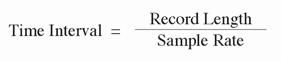
Time Interval
Oscilloscopes allow you to select record length to optimize the level of detail needed for your application. If you are analyzing an extremely stable sinusoidal signal, you may need only a 500 point record length, but if you are isolating the causes of timing anomalies in a complex digital data stream, you may need a million points or more for a given record length, as shown in Figure 51.

Figure 51: Capturing the high frequency detail of this modulated 85 MHz carrier requires high resolution sampling (100 ps). Seeing the signal's complete modulation envelope requires a long time duration (1 ms). Using long record length (10 MB), the oscilloscope can display both.
Triggering Capabilities
An oscilloscope's trigger function synchronizes the horizontal sweep at the correct point of the signal. This is essential for clear signal characterization. Trigger controls allow you to stabilize repetitive waveforms and capture single-shot waveforms.
Effective Bits
Effective bits represent a measure of a digital oscilloscope's ability to accurately reconstruct a sine wave signal's shape. This measurement compares the oscilloscope's actual error to that of a theoretical “ideal” digitizer. Because the actual errors include noise and distortion, the frequency and amplitude of the signal must be specified.
Frequency Response
Bandwidth alone is not enough to ensure that an oscilloscope can accurately capture a high frequency signal. The goal of oscilloscope design is a specific type of frequency response: maximally flat envelope delay (MFED). A frequency response of this type delivers excellent pulse fidelity with minimum overshoot and ringing. Since a digital oscilloscope is composed of real amplifiers, attenuators, ADCs, interconnects, and relays, MFED response is a goal that can only be approached. Pulse fidelity varies considerably with model and manufacturer.
Vertical Sensitivity
Vertical sensitivity indicates how much the vertical amplifier can amplify a weak signal. This is usually measured in millivolts (mV) per division. The smallest voltage detected by a general-purpose oscilloscope is typically about 1 mV per vertical screen division.
Sweep Speed
Sweep speed indicates how fast the trace can sweep across the oscilloscope screen, making it possible to see fine details. The sweep speed of an oscilloscope is represented by time (seconds) per division.
Gain Accuracy
Gain accuracy indicates how accurately the vertical system attenuates or amplifies a signal, usually represented as a percentage error.
Horizontal Accuracy (Time Base)
Horizontal accuracy, or time base accuracy, indicates how accurately the horizontal system displays the timing of a signal, usually represented as a percentage error.
Vertical Resolution (Analog-to-Digital Converter)
Vertical resolution of the analog-to-digital converter (ADC), and therefore, the digital oscilloscope, indicates how precisely it can convert input voltages into digital values. Vertical resolution is measured in bits. Calculation techniques can improve the effective resolution, as exemplified with hi-res acquisition mode.
Timing Resolution Mixed Signal Oscilloscopes (MSO)
An important MSO acquisition specification is the timing resolution used for capturing digital signals. Acquiring a signal with better timing resolution provides a more accurate timing measurement of when the signal changes. For example, a 500 MS/s acquisition rate has 2 ns timing resolution and the acquired signal edge uncertainty is 2 ns. A smaller timing resolution of 60.6 ps (16.5 GS/s) decreases the signal edge uncertainty to 60.6 ps and captures faster changing signals.
Some MSOs internally acquire digital signals with two types of acquisitions at the same time. The first acquisition is with standard timing resolution, and the second acquisition uses a high-speed resolution. The standard resolution is used over a longer record length while the high-speed timing acquisition offers more resolution around a narrow point of interest (Figure 52).

Figure 52: The MSO provides 16 integrated digital channels, enabling the ability to view and analyze time-correlated analog and digital signals. A high speed timing acquisition provides more resolution to reveal narrow events such as glitches.
Connectivity
The need to analyze measurement results remains of utmost importance. The need to document and share information and measurement results easily and frequently has also grown in importance. The connectivity of an oscilloscope delivers advanced analysis capabilities and simplifies the documentation and sharing of results. As shown in Figure 53, standard interfaces (GPIB, RS-232, USB, and Ethernet) and network communication modules enable some oscilloscopes to deliver a vast array of functionality and control.

Figure 53: Today's oscilloscopes provide a wide array of communications interfaces, such as a standard Centronics port and optional Ethernet/RS-232, GPIB/RS-232, and VGA/RS-232 modules. There is even a USB port (not shown) on the front panel.
Some advanced oscilloscopes also let you:
- Create, edit and share documents on the oscilloscope, all while working with the instrument in your particular environment
- Access network printing and file sharing resources
- Access the Windows® desktop
- Run third-party analysis and documentation software
- Link to networks
- Access the Internet
- Send and receive e-mail
Expandability
An oscilloscope should be able to accommodate your needs as they change. Some oscilloscopes allow you to:
- Add memory to channels to analyze longer record lengths
- Add application-specific measurement capabilities
- Complement the power of the oscilloscope with a full range of probes and modules
- Work with popular third-party analysis and productivity
- Windows-compatible software
- Add accessories, such as battery packs and rack mounts
Application modules and software may enable you to transform your oscilloscope into a highly-specialized analysis tool capable of performing functions such as jitter and timing analysis, microprocessor memory system verification, communications standards testing, disk drive measurements, video measurements, power measurements and much more. Figures 54 through 59 highlight a few of these examples.

Figure 54: Analysis software packages are specifically designed to meet jitter and eye measurement needs of today's high-speed digital designers.

Figure 55: Serial bus analysis is accelerated with automated trigger, decode, and search on serial packet context.

Figure 56: Advanced DDR analysis tools automate complex memory tasks like separating read/write bursts and performing JEDEC measurements.

Figure 57: Video application modules make the oscilloscope a fast, tell-all tool for video troubleshooting.

Figure 58: Advanced analysis and productivity software, such as MATLAB®, can be installed in Windows-based oscilloscopes to accomplish local signal analysis.