A Revolutionary Tool for Signal Discovery, Trigger, Capture and Analysis
Detection is the first step in characterizing, diagnosing, understanding and resolving any problem relating to timevariant signals. As more channels crowd into available bandwidth, new applications utilize wireless transmission, and RF systems become digital-based, engineers need better tools to help them find and interpret complex behaviors and interactions.
Tektronix patented Digital Phosphor technology, or DPX®, is used in our Real-Time Spectrum Analyzers (RSAs) to reveal signal details that are completely missed by conventional spectrum analyzers and vector signal analyzers. The full-motion DPX Live RF spectrum display shows signals never seen before, giving users instant insight and greatly accelerating discovery and diagnosis. DPX is standard on all Tektronix RSAs. With the recently introduced, real-time DPX TimeDomain display technology, Tektronix Real-Time Spectrum Analyzers now become Real-Time Signal Analyzers.
This primer describes the methods behind the DPX Live RF spectrum display, swept DPX, Time-Domain DPX Displays, DPX Density™ measurements, DPX Density™ and Frequency Edge triggers.
- Swept DPX revolutionizes spectrum analysis by enlarging the DPX span to cover the instrument's entire frequency range. The analyzer acquires a wide span as a series of realtime segments, each tens of megahertz wide, merging them into a complete DPX Spectrum graph.
- Time-Domain DPX transform real-time viewing from spectrum viewing to methods of analysis for detailed signal analysis. With real-time views of amplitude (Zero Span), phase, and frequency versus time at update rates that are orders of magnitude faster than conventional signal analyzers.
- DPX Density™ trigger is a completely new way to catch the signals you discover with the DPX Spectrum display. In many cases, it is the only way to capture signals hiding beneath other signals. While just seeing these signals in the DPX display is sometimes enough to set you on the track to diagnosis, it is often important to acquire a data record of the signal for further analysis.
- Frequency Edge trigger provide another unique method of signal isolation that runs concurrently within the DPX engine to isolate signal transition at a specific frequency and threshold. By combining this functionality with trigger interpolation, you now have a unique, low jitter, method for analyzing signal frequency transitions.
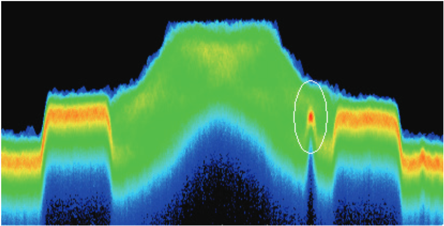
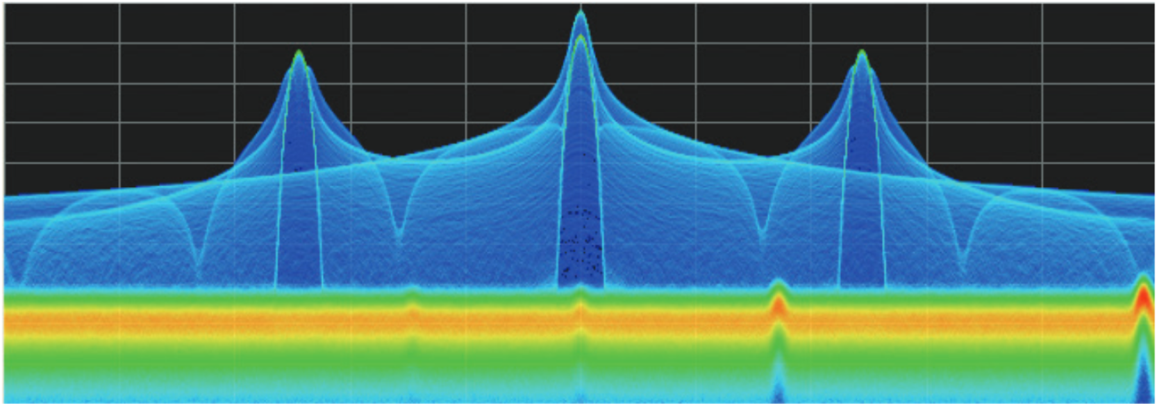
One example, Figure 1, demonstrates a hard-to-catch signal is an unexpected narrow-band transmission buried in the FM signal. No previous method for triggering in the time or frequency domain will enable the event triggering and isolation of this event. DPX Density trigger now enables a method for triggering on the persistency (or time density) of the signal.
Additional advancements in DPX performance and functionality include major increases in speed and z-axis resolution. Faster spectral transforms (>290,000 per second) guarantee display of events as short as 3.7 µsec, plus better visual representation of transient signals. Higher resolution in the Z axis provides accurate measurements of signal density at any frequencyamplitude point in the DPX Spectrum graph. Color scaling for the density axis has been enhanced by the addition of useradjustable mapping.
One-click automation features will have you using these valuable new capabilities within minutes of turning on your new or upgraded instrument. The first of these is Auto Color, which quickly adjusts the color range of the DPX bitmap for whatever signals are currently displayed. The other is Trigger On This™, a pop-up menu selection that turns on DPX Density triggering and sets its parameters to capture the signal you clicked on.
DPX capabilities and features referenced in this primer may not be available in all Tektronix spectrum analyzers. The functionality described in this document is representative of a fully equipped RSA5000 and RSA6000 Series spectrum analyzers equipped with Option 200.
The DPX Display
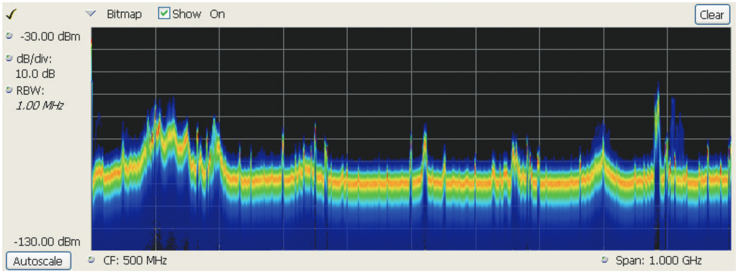
With the DPX Spectrum display you can detect and accurately measure transients as brief as 3.7 µsec. Dedicated hardware computes up to 292,000 spectrums per second on the digitized input signal. Then it displays all these spectrums as a colorgraded bitmap that reveals low-amplitude signals beneath stronger signals sharing the same frequency at different times.
The strong signal in the DPX spectrum graph, shown in Figure 2, is a repeating pulse at a fixed frequency. There is also a lower-power CW signal that steps very quickly through the same span. During the pulse's on time, the power of the two signals is additive, resulting in nearly undetectable differences in the pulse envelope shape. But during the time the pulse is off, the sweeping signal is detected and shown in its true form. Both signals are visible in the bitmap because at least one full cycle of their activities occurs within a single DPX display update.
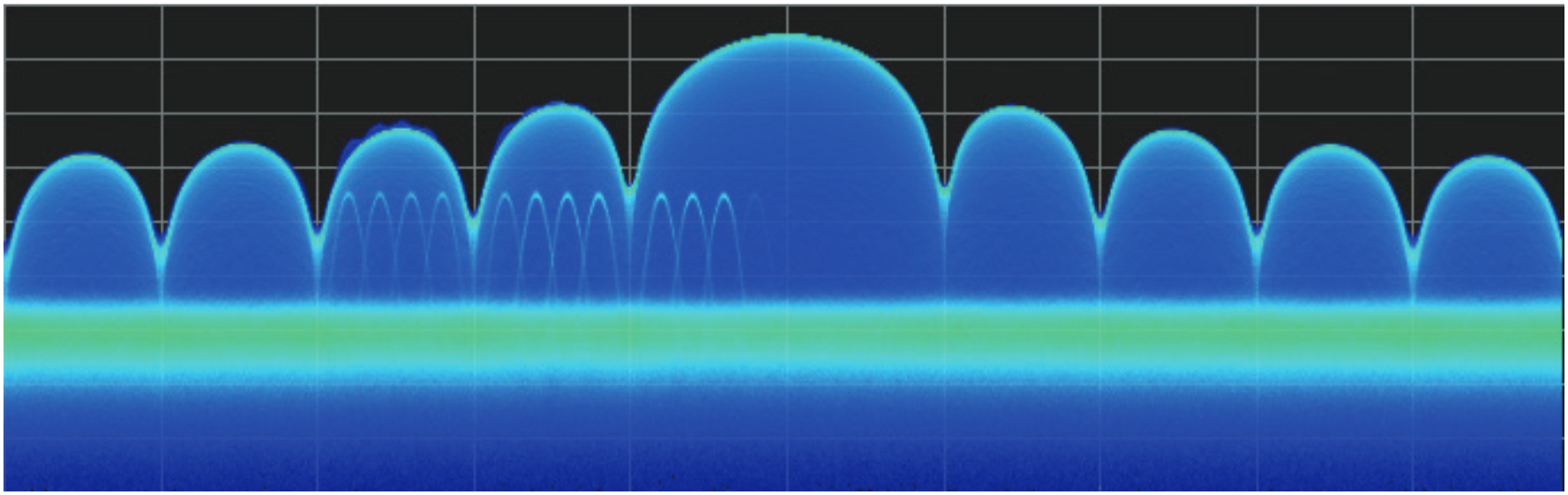
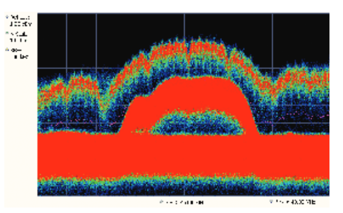
Compare the display of a traditional swept spectrum analyzer (Figure 3) and that of a real-time spectrum analyzer with a DPX spectrum display (Figure 4). The signal captured is a typical WLAN interchange between a nearby PC and a more-distant network access point (AP). The laptop signal is nearly 30 dB stronger than the AP's signal because it is closer to the measuring antenna.
The traditional swept spectrum analyzer display, Figure 3, uses line traces that can show only one level for each frequency point, representing the largest, the smallest or the average power. After many sweeps, the Max Hold trace shows a rough envelope of the stronger laptop signal. +Peak detection was selected for the other trace in an attempt to capture the weaker but more frequent AP signal, but the bursts are very brief, so the likelihood of seeing one in any particular sweep is small. It will also take a long time to statistically capture the entire spectrum of a bursted signal due to the architecture of the swept spectrum analysis.
The DPX spectrum display, Figure 4, reveals much more insight on the same signal. Since it is a bitmap image instead of a line trace, you can distinguish many different signals occurring within each update period and/or different version of the same signal varying over time. The heavy band running straight across the lower third of the graph is the noise background when neither the laptop nor the AP is transmitting. The red lump of energy in the middle is the ON shape of the AP signal. Finally, the more delicate spectrum above the others is the laptop transmissions. In the color scheme used for this demonstration ("Temperature"), the hot red color indicates a signal that is much more frequent than signals shown in cooler colors. The laptop signal, in yellow, green and blue, has higher amplitude but doesn't occur nearly as often as the AP transmissions because the laptop was downloading a file when this screen capture was taken.
Behind the Scenes: How DPX Works
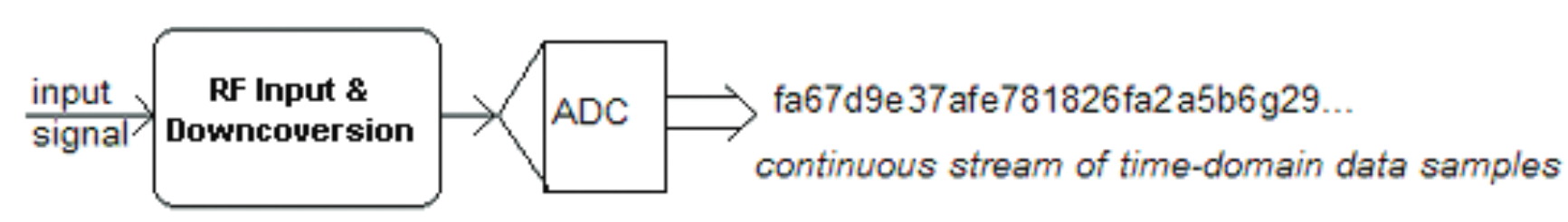
This section explains how DPX spectrum displays are created. The input RF signal is conditioned and down-converted as usual for a spectrum analyzer, then digitized. The digitized data is sent through an FPGA that computes very fast spectral transforms, and the resulting frequency-domain waveforms are rasterized to create the bitmaps.
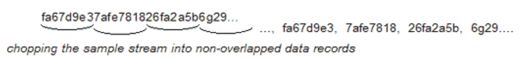
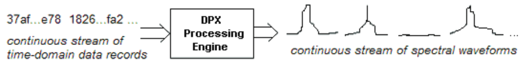
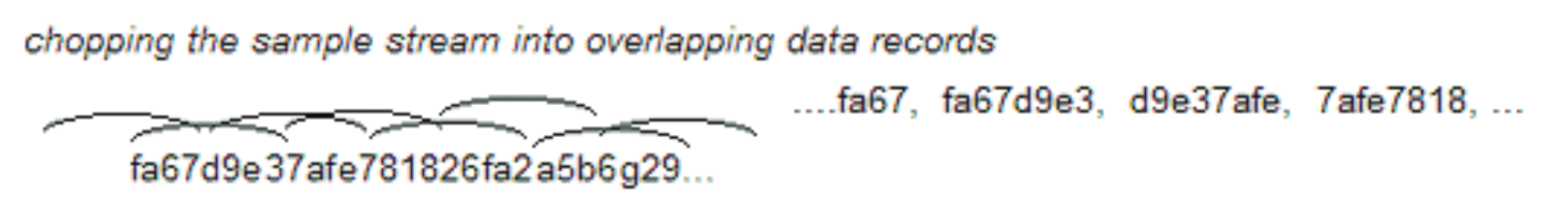
The DPX bitmap that you see on screen is composed of pixels representing x, y, and z values for frequency, amplitude, and hit count (some instruments can be upgraded to enable the z-axis measurement Density in place of hit count). A multi-stage process, shown in Figures 5a - 5d, creates this bitmap, starting with analog-to-digital conversion of the input signal.
Collecting Spectral Data
- RF signals are downconverted and sampled into a continuous data stream.
- Samples are segmented into data records for FFT processing based on the selected resolution bandwidth.
- Data records are process in DPX transform engine.
- For some products, over-lapped FFT processing is used to improve minimum event duration performance.
As long as spectral transforms are performed faster than the acquisition data records arrive, the transforms can overlap each other in time, so no events are missed in between. Minimum event length for guaranteed capture depends on the length of the data records being transformed. An event must last through two consecutive data records in order for its amplitude to be accurately measured. Shorter events are detected and visible on screen, but may be attenuated. The DPX Spectrum RBW setting determines the data record length; narrow RBW filters have a longer time constant than wide RBW filters. This longer time constant requires longer FFTs, reducing the transform rate. Additional detail on minimum signal duration is provided in "Guaranteed Capture of Fast Events" later in this primer.
The spectral waveforms are plotted onto a grid of counting cells called the "bitmap database". The number held by each database cell is the z-axis count. For simplicity, the small example grid used here in Figure 6 is 11x10, so our spectral waveforms will each contain 11 points. A waveform contains one (y) amplitude value for each (x) frequency. As waveforms are plotted to the grid, the cells increment their values each time they receive a waveform point.
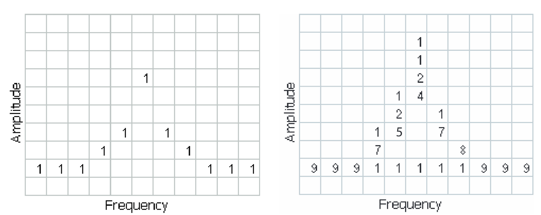
The grid on the left shows what the database cells might contain after a single spectrum is plotted into it. Blank cells contain the value zero, meaning that no points from a spectrum have fallen into them yet.
The grid on the right shows values that our simplified database might contain after an additional eight spectral transforms have been performed and their results stored in the cells. One of the nine spectrums happened to be computed as a time during which the signal was absent, as you can see by the string of "1" occurrence counts at the noise floor.
Frame Updates
The maximum rate for performing the variable-length frequency transforms that produce those waveforms can be greater than 292,000 per second. Measurement settings that slow this transform rate include narrowing the RBW and increasing the number of points for the line traces available in the DPX Spectrum display along with the bitmap. Even at their slowest, spectral transforms are performed orders of magnitude faster than a physical display can respond, and also too fast for humans to see, so there's no need to update the screen or measurements at this rate. Instead, the grid collects thousands of waveforms into "frames", each covering about 50 milliseconds (ms). A 50 ms frame contains the counts from up to 14,600 waveforms. After each frame's waveforms have been mapped into the grid, the cell occurrence counts are converted to colors and written to the DPX bitmap, resulting in a bitmap update rate of around 20 per second.
Frame length sets the time resolution for DPX measurements. If the bitmap shows that a -10 dBm signal at 72.3 MHz was present for 10% of one frame's duration (5 msec out of 50 msec), it isn't possible to determine just from the DPX display whether the actual signal contained a single 5 ms pulse, one hundred 50 microsecond (µs) pulses, or something in between. For this information, you need to examine the spectral details of the signal or use another display with finer time resolution, such as Frequency vs. Time or Amplitude vs. Time.
Converting Occurrence Counts to Color
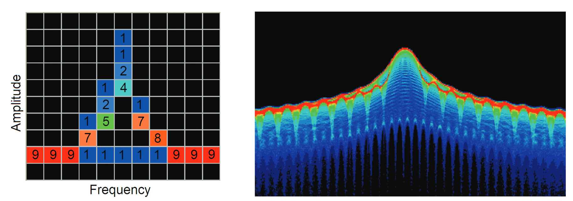
About 20 times per second, the grid values are transferred to the next process step, in which the z-axis values are mapped to pixel colors in the visible bitmap, turning data into information (Figure 7). In this example, warmer colors (red, orange, yellow) indicate more occurrences. The color palette is user-selectable, but for now we will assume the default "temperature" palette.
The result of coloring the database cells, Figure 8, according to the number of times they were written into by the nine spectrums, one per pixel on the screen, creates the spectacular DPX displays.
Adjusting the Minimum above the black default allows you to concentrate most of your color resolution over a small range of medium or higher occurrence rates to visually discriminate between different signals that have nearly equal probability values.
To see why adjustable color scaling is useful compare Figures 9 and 10. On the Scale tab, the Max control to is set to 100% in Figure 9. The range of colors now covers the full z-axis range of densities from 0 to 100%. The signals used to create this bitmap are fairly diffuse in both frequency and amplitude, so most pixels have low occurrence counts or density values, so the upper half of the color palette is unused.
When the Auto Color button is selected, this the Maximum control to the highest pixel value in the current bitmap in Figure 10. Now none of the available colors remain unused. The entire palette is mapped to the occurrence values present at the time the button is selected, providing better visual resolution for low densities. Selecting the Autoscale button in the DPX display scales all three axes based on current results.
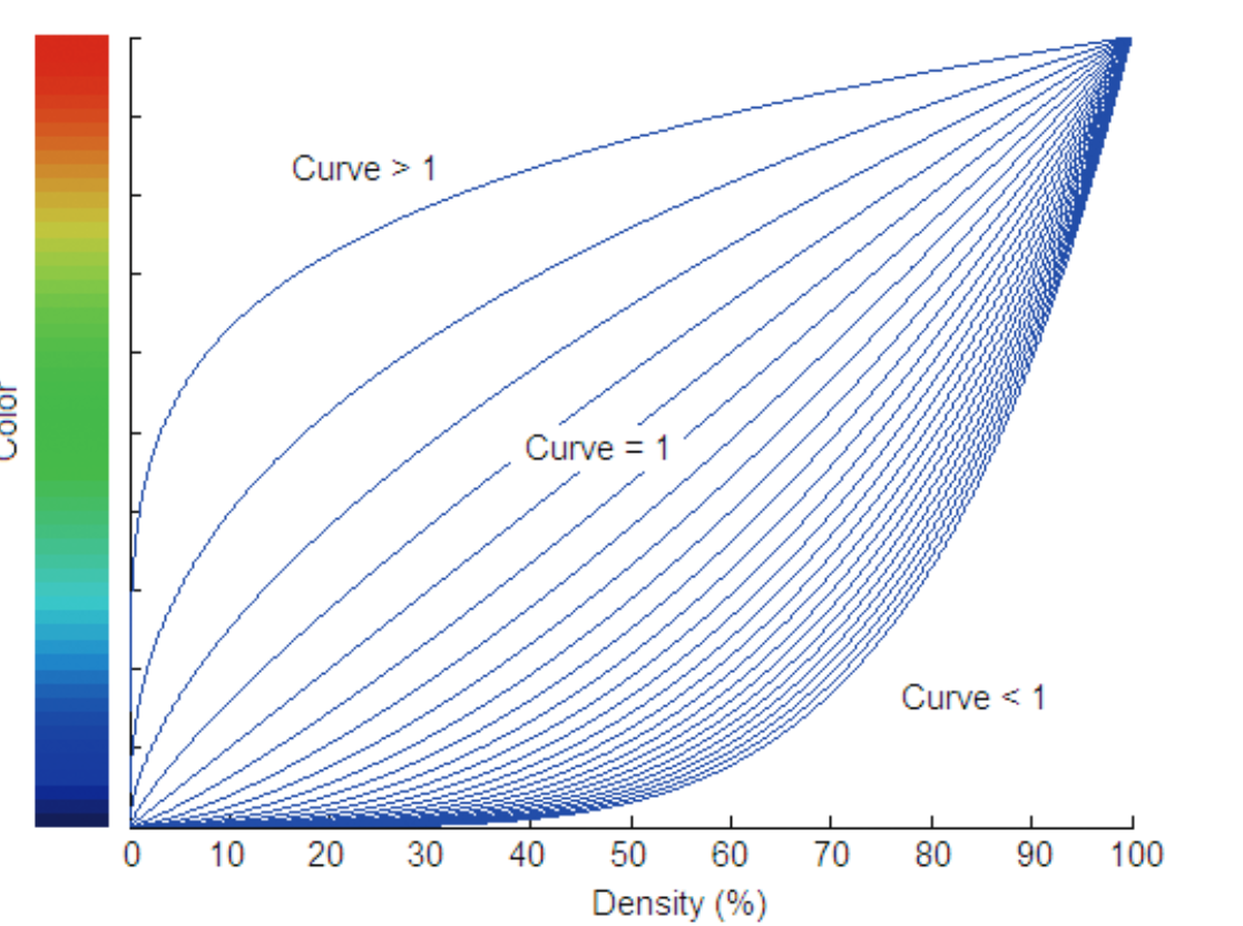
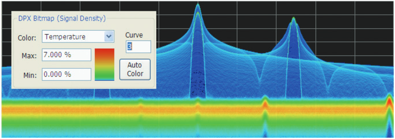
Color Mapping Curves
The mapping between z-axis values and color doesn't have to be linear. The Curve control lets you choose the shape of the mapping equation. A Curve setting of 1 selects the straight-line relationship. Higher Curve numbers pull the curve upwards and to the left, concentrating color resolution on lower densities. Settings less than 1 invert the curve, moving the focus of the color range towards higher density values. Figure 11 shows the mapping curves.
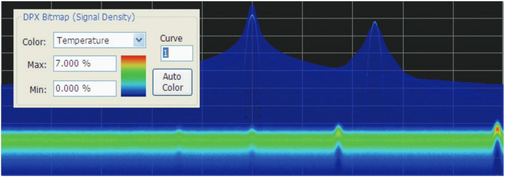
Using the same example demonstrated in Figures 9 and 10 analyzing the on the impact of adjusting the color scale, the impact of setting the curve control can be observed. With the Curve control set to 1 in the Scale tab, shown in Figure 12, one can observe how the color palette illustration to the left of the Curve control changes as the Curve is varied. When the mapping is linear, the colors spread evenly across the full density range.
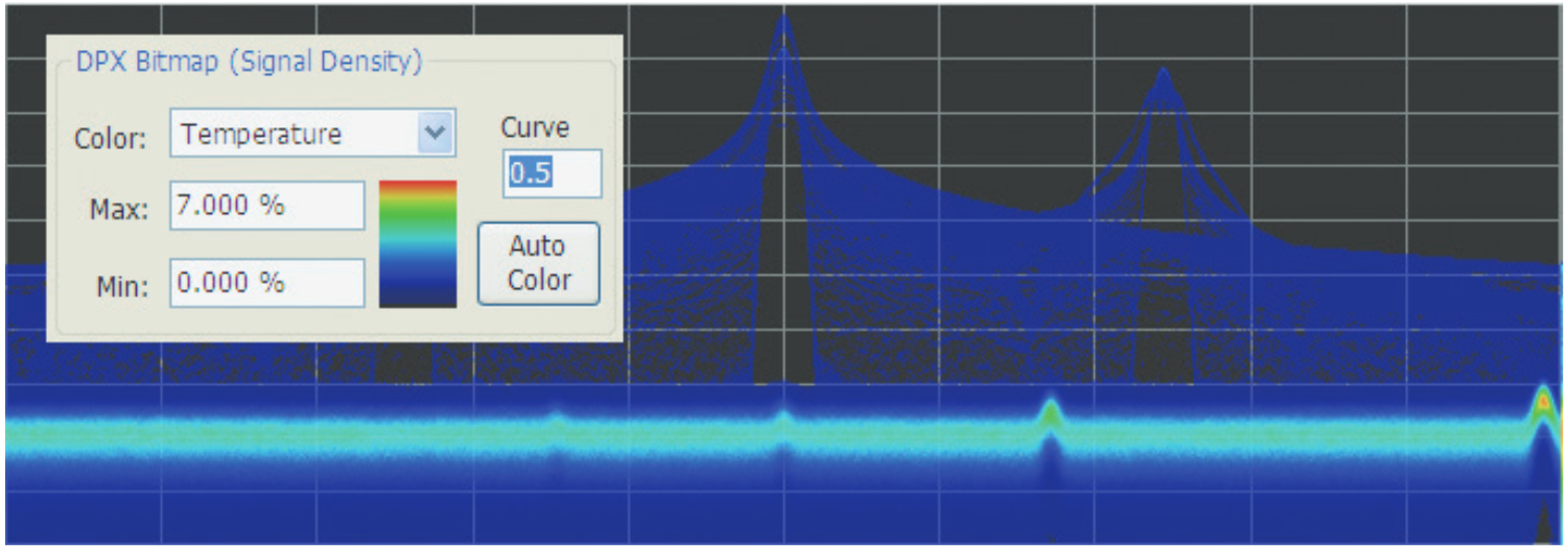
When the Curve control is set to 0.5, as shown in Figure 13, the best color resolution is in the upper half of the density range, and only the dark blues are assigned to densities below 50%.
In Figure 14, the Curve control is increase to 3. The majority of colors shifts to the lower half of the density scale, but various shades of orange and red are still available for densities above 50%.
Swept DPX
DPX Spectrum is not limited in span by its real-time bandwidth. Like the regular Spectrum display, DPX Spectrum steps through multiple real-time frequency segments, building a wide-span display with line traces and the bitmap.
The analyzer "dwells" in each frequency segment for one or more DPX frames, each containing the results of up to 14,600 spectral transforms. Dwell time is adjustable, so you can monitor each segment of the sweep for up to 100 seconds before moving to the next step. While dwelling in a segment, the probability of intercept for signals within that frequency band is the same as in normal, real-time spans: 100% capture of events as short as 3.7 µsec.
A full pixel bitmap is created for every segment and compressed horizontally to the number of columns needed for displaying the frequency segment. Compression is done by averaging pixel densities of the points being combined together. The final swept bitmap contains a representation of the same pixel bitmap resolution, just like the non-swept bitmaps. Line traces are also created in full for each segment, and then horizontally compressed to the user-selected number of trace points for the full span.
A complex algorithm for determining the number and width of each frequency segment has been implemented. The variables in the equation include user-adjustable control settings like Span, RBW, and number of trace points, RF and IF optimization, and Acquisition BW. Installed hardware options also can affect the span segmentation. The number of segments ranges from 10 to 50 for each 1 GHz in a sweep.
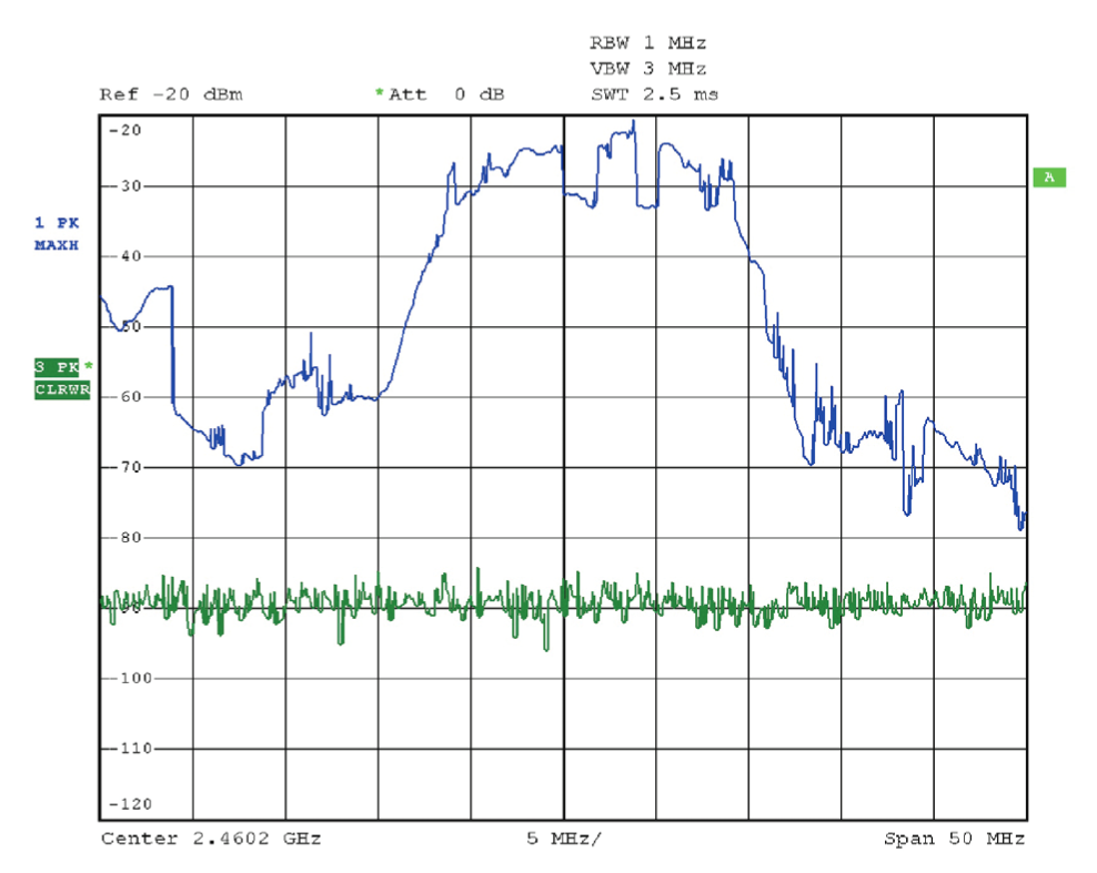
A helpful piece of information for operators is the actual Acquisition Bandwidth used for capturing each segment. "Acq BW" is shown in the Acquire control panel on the Sampling Parameters tab. Acq BW is typically set automatically by the instrument, based on the needs of all the open displays, but can also be set manually. In either case, the displayed bandwidth is used for every frequency segment in the swept DPX display. The width of the segments is optimized for performance.
The entire instrument frequency range of many GHz can be covered in a DPX sweep. A simple control allows the amount of time DPX spends in each segment. This control, circled in Figure 16, can be set between 50 ms and 100 seconds.


DPX Time-Domain Displays
Like the original DPX Spectrum display, the DPX Time-domain displays reinvent a previously-existing instrument capability by increasing the measurement rate by several orders of magnitude and adding powerful new DSP-based functions. These new time-domain displays employ the DPX processing engine to produce Amplitude, Frequency or Phase vs. time.
DPX Zero Span is a higher-performance version of the traditional zero-span feature of swept spectrum analyzers. DPX Frequency and Phase displays plot the input signal’s instantaneous frequency and phase values as a function of time, in the same manner that Zero Span plots instantaneous amplitude values vs. time.
The preceding section of this primer, "Behind the Scenes: How DPX Spectrum Works", largely applies to the DPX time-domain displays as well. Just like DPX Spectrum, the DPX time-domain displays contain both bitmap and trace data. The bitmap display is color-graded with adjustable persistence, like the bitmap display for DPX Spectrum.
The fundamental differences between the DPX frequency- and time-domain displays are:
- An FFT is not used for time-domain displays. Instead, the digitized data remains in the time domain. For the Frequency and Phase displays, the data is converted to frequency or phase.
- Additional filtering can be done on the time-domain data, replacing the RBW filter used in DPX Spectrum.
- Instead of being continuously generated as in DPX Spectrum, data for the time-domain DPX displays can be captured in response to trigger events, like an oscilloscope, though free-run is also supported.*1
- The frame update rate decreases when triggers are occurring infrequently or the sweep time is long.
In many respects, the DPX time-domain circuit acts like an oscilloscope, plotting signal values over time. Familiar oscilloscope controls, such as vertical scale and position, sweep speed, zoom and pan, are present in DPX Time Domain displays, and work the same as they do in scopes.
Analyzing Amplitude, Frequency, or Phase
DPX time-domain processing starts with the same downconverted data used by DPX Spectrum and all the analyzer’s other measurements. The input signal is in I-Q format after down-conversion. If additional bandwidth reduction is desired, a filter is applied to the I-Q data stream. Next, a CORDIC*2 converts the I-Q data to phase and amplitude. For magnitude displays (dB, Volts, Watts) the amplitude data from the CORDIC is used to produce a time-domain waveform that is placed in the bitmap and traces.
For phase and frequency displays, only the phase data is used. Phase data from the CORDIC is initially converted to frequency by a simple differentiator, taking the difference from one phase sample to the next. All filtering and data processing is done on this frequency waveform, then for phase waveforms, the final step is an integration (taking the sum of all consecutive samples) to obtain the phase data.*3
Traces, Frames and Sweep
Similar to DPX spectrum, traces are produced from the samples of incoming data, and these traces are written to a bitmap and color-graded according to their signal density over the period of a frame. One or more traces are used to create a frame, which is what the DPX engine sends to the display. Frames contain multiple traces when DPX is computing traces faster than the display can catch them. For longer time sweeps, frame length is either extended, or multiple frames are seamlessly stitched in time to create the display. Several methods for compressing and viewing the data are available as described below.
>Traces and bitmaps
A trace is produced every time the DPX engine processes data, either as the result of trigger or upon receiving a freerun command from the triggering system. A trace has had bandwidth processing applied and its points have been converted to amplitude, frequency or phase. The traces are collected by the DPX engine and converted to the color bitmap for a frame. When sweep times are less than 1 second, traces are placed into a single frame and sent to the screen at a variable rate.
Frame Updates
New data frames are sent to the display system at a maximum rate of 20 times each second (50 ms/frame). If the sweep time is greater than 50 ms and less than 1 second, the DPX frame time is extended to match the sweep time. Like DPX Spectrum frames, every time-domain frame includes the bitmap and three user-selectable traces. The bitmap resolution of 801x201 is the same as for DPX Spectrum, but the time-domain traces are always 801 samples long, whereas trace length is adjustable in DPX Spectrum.
When a sweep (acquisition) takes 50 ms or longer, it isn’t possible to have multiple sweeps in a single frame, because a single acquisition takes more time than an entire frame normally needs, and the frame ends up waiting for the acquisition to complete before it updates the screen. This is also the case when the time between trigger events is 50 ms or more.
Fast Sweeps
When sweeps (acquisitions) are happening faster than frames can be generated (20/sec, or 50 ms/sweep), each frame contains the results from multiple acquisitions. The acquisitions each yield one trace, and all the traces collected over 50 msec are combined into the frame’s bitmap and line traces. The number of acquisitions in a single frame ranges from 1 to more than 2,500, depending on sweep time and trigger rate. This results a maximum trace update rate in excess of 50,000 waveforms per second for sweep times less than or equal to 10 µs.
If you want to capture one trigger event with each acquisition, with minimum dead time waiting for the next trigger to occur, set your sweep time a bit shorter than the time between trigger events.
Slow Sweeps
For "slow" sweeps (typically 1 second and longer), the frame rate is always 20/second. Multiple trace segments are placed end-to-end across the screen to create the complete sweep. This incremental updates mode creates the following three types of displays:
- Free Run / Normal Trace Motion - The bitmap and traces are built up from the left edge of the graph. New points are added the right of previous points at the selected sweep rate. Once the display has filled, the display starts sweeping from the left edge again. New points overwrite those from the previous sweep, erasing the old data from memory.
- Free Run / Roll - New bitmap and trace points appear at the right edge of the display and slide towards the left as new points arrive to displace them. Once data points have disappeared off the left edge of the graph, they are no longer in memory.
- Triggered - While waiting for the trigger event, the display acts like Free Run / Roll, but with the new data points appearing at the trigger location rather than at the right edge of the graph. Points slide from the trigger location towards the left edge as each new point arrives. Once a trigger event is recognized, the post-trigger data points are added to the right of the trigger point, as in Free Run / Normal Trace Motion. When the trace has filled in all the way to the right edge of the graph, the sweep starts over again.
When DPX Time-Domain is in Free Run, the user can select either Normal or Roll trace motion (#1 or #2 above). In Triggered mode, method #3 is used to display the sweep.
*1 In DPX Spectrum, the FFT runs continuously whether the trigger mode is Free Run or Triggered, and at the hardware level the DPX bitmap and traces are always being generated When the display is set to "DPX shows only trigger frames", the screen is only updated in response to trigger events and frames that don’t contain triggered data are not shown. In DPX Time Domain, the bitmap and traces do not receive new data unless a trigger occurs or the display is in Free Run. This can affect both the display update rate and bitmap persistence.
*2 Coordinate Rotation Digital Computer: a hardware-efficient algorithm for computation of trigonometric functions.
*3 Waiting to compute the phase after all the filtering allows the phase display to wrap at +-180 degrees without affecting the signal passing through the filters.
Find more valuable resources at TEK.COM
Copyright © Tektronix. All rights reserved. Tektronix products are covered by U.S. and foreign patents, issued and pending. Information in this publication supersedes that in all previously published material. Specification and price change privileges reserved. TEKTRONIX and TEK are registered trademarks of Tektronix, Inc. All other trade names referenced are the service marks, trademarks or registered trademarks of their respective companies.
01/17 37W-17249-6